

Abstract
Recent research has quantified the contributions of CO2 and CH4 emissions traced to the products of major fossil fuel companies and cement manufacturers to global atmospheric CO2, surface temperature, and sea level rise. This work has informed societal considerations of the climate responsibilities of these major industrial carbon producers. Here, we extend this work to historical (1880–2015) and recent (1965–2015) acidification of the world's ocean. Using an energy balance carbon-cycle model, we find that emissions traced to the 88 largest industrial carbon producers from 1880–2015 and 1965–2015 have contributed ∼55% and ∼51%, respectively, of the historical 1880–2015 decline in surface ocean pH. As ocean acidification is not spatially uniform, we employ a three-dimensional ocean model and identify five marine regions with large declines in surface water pH and aragonite saturation state over similar historical (average 1850–1859 to average 2000–2009) and recent (average 1960–1969 to average of 2000–2009) time periods. We characterize the biological and socioeconomic systems in these regions facing loss and damage from ocean acidification in the context of climate change and other stressors. Such analysis can inform societal consideration of carbon producer responsibility for current and near-term risks of further loss and damage to human communities dependent on marine ecosystems and fisheries vulnerable to ocean acidification.
Export citation and abstract BibTeX RIS
1. Introduction
The question of responsibility for climate change is central to the consideration of societal obligations to address the problem. International climate policy frameworks focus on the climate responsibilities of nations. Article 2.2 of the Paris Agreement sets forth that the terms of the Agreement will be implemented by nations that are Parties to it, 'to reflect equity and the principle of common but differentiated responsibilities and respective capabilities.' (United Nations 2015).
Climate responsibilities extend well beyond national governments. Sub-national governments, corporations, utilities, and individuals often see themselves, and are viewed by others, as having obligations to address climate change. Societal perceptions that fossil fuel companies bear distinctive climate responsibilities are reflected in the emergence of divestment campaigns (Stephens et al 2018), shareholder resolutions seeking alignment of company practices with the Paris Agreement (Fugere and Behar 2018, Millar et al 2018), and litigation. In 2017 and 2018, for example, more than a dozen US cities and counties and the state of Rhode Island filed suit against several investor-owned fossil fuel companies seeking to hold them liable for their contributions to the harms from sea level rise and increasingly extreme weather that climate change is imposing on local communities (Hasemyer 2018). In 2018, the Pacific Coast Federation of Fishermen's Association filed suit against fossil fuel companies for harms from the ocean warming linked with a buildup of domoic acid in Dungeness crabs at levels toxic for human consumption (Bond et al 2015, Zhu et al 2017, Hulac 2018).
Societal consideration of the climate responsibilities of fossil fuel companies can also be informed by scholarly research. Recent studies have documented that the fossil fuel industry was broadly aware of the climate risks of their products since at least the mid-1960s (Franta 2018), and that some companies sought to publicly discredit climate science and known climate risks (Frumhoff et al 2015, Supran and Oreskes 2017) while taking steps to protect company assets from these risks.
Recent research has also quantified the large contribution of fossil fuel company-traced emissions to the problem. Heede (2014) found that nearly two-thirds of all industrial carbon dioxide (CO2) and methane (CH4) emissions between 1880 and 2010 can be traced to the products of 83 large producers of coal, oil, and natural gas, and 7 cement manufacturers. Incorporating Heede's (2014) database into a simple climate model, Ekwurzel et al (2017) found that between 1880 and 2010, emissions traced to these 90 largest industrial carbon producers contributed ∼57% of the rise in atmospheric CO2, 42%–50% of the rise in global mean surface temperature, and approximately 26%–32% of the rise in global sea level.
Here, we quantify the contribution of CO2 emissions traced to major industrial carbon producers to global-scale ocean acidification. This may inform societal consideration of carbon producer responsibility for loss and damage to human communities dependent upon marine ecosystems and fisheries vulnerable to ocean acidification. We examine the effects of these emissions on global ocean surface water pH over two time-periods: 1880–2015, the historical period with robust emission data available (Heede 2014, supplementary material table 7 is available online at stacks.iop.org/ERL/14/124060/mmedia), and a more recent period of 1965–2015, roughly consistent with the period when major fossil fuel companies were increasingly aware that continued emissions from the use of their products posed significant climate risks (Franta 2018).
Ocean acidification resulting from rising atmospheric CO2 is already having and is expected to have further fundamental and substantial impacts on a wide variety of marine organisms, including ecosystems and fisheries with significant economic and cultural value (Cooley and Doney 2009, Doney et al 2009, Feely et al 2009, Gattuso et al 2015, Hoegh-Guldberg et al 2019). Oceanic surface waters currently absorb approximately one quarter of the additional carbon dioxide introduced to the atmosphere by anthropogenic emissions, increasing the partial pressure of carbon dioxide in surface waters (Doney et al 2014, Gruber et al 2019). Over a recent decade (2008–2017), the ocean absorbed approximately 2.4 +/−0.5 GtCyr−1 (Le Quéré et al 2018). A series of chemical reactions leads to a higher concentration of hydrogen and bicarbonate ions, and a lower concentration of carbonate ions, which together result in reduced pH and carbonate mineral saturation states (Zeebe and Wolf-Gladrow 2001, Feely et al 2004).
The ocean is now acidifying at a rate unparalleled in the last 66 million years (Zeebe et al 2016); since pre-industrial times, ocean surface water pH has decreased on average by about 0.1 pH units, an increase in acidity of ∼26%. The saturation state of aragonite, an indicator of ocean acidification, has decreased on average by ∼0.5, or ∼17%, with substantial latitudinal variations (Feely et al 2009, IPCC 2014). As documented previously (e.g. Feely et al 2009), ocean acidification is not spatially uniform: regional ocean acidification signals reflect a combination of air-sea gas exchange and ocean circulation patterns along with temperature dependence on seawater CO2 thermodynamics, which lead to differences between pH and aragonite saturation state responses.
Marine species and ecosystems that benefit people have already been harmed by ocean acidification. Laboratory studies have shown that CO2-driven acidification decreases calcification among mollusks, crustaceans, stony corals, and coralline algae, reduces the survival of juvenile mollusks and crustaceans (Kroeker et al 2013, Bednaršek et al 2016), and decreases reproductive success for many species, including corals (Albright et al 2010). Oyster hatcheries in the United States have experienced heightened larval shellfish mortality due to acidification (Barton et al 2015, 2012), depressing industry revenues in the Pacific Northwest and endangering over 3000 jobs in Washington state during the mid-2000s. After investments in adaptation measures, the industry has largely recovered. Ocean acidification also alters the development and behavior of many finfish (e.g. clownfish, dusky sharks, rockfish, summer flounder) in laboratory studies (Munday et al 2009, Chambers et al 2013, Hamilton et al 2014, Dixson et al 2015).
The impacts of ocean acidification (Pershing et al 2018) take place in the context of other changes to the ocean's physical and chemical properties that are tied to carbon emissions. These include changes to sea surface temperatures, salinity, oxygen levels, and circulation patterns (Bindoff et al 2013, Hill et al 2015, Ekwurzel et al 2017). As the ocean has acidified, it has also absorbed most of the excess heat produced through global warming, increasing sea surface temperatures by ∼0.9 °C above pre-industrial levels (IPCC 2018). The Great Barrier Reef and other warm-water coral reef ecosystems, for example, are already being harmed by a combination of warming and acidification (Albright et al 2016, IPCC 2018). Natural variability combined with warming ocean waters means high temperature events are more frequently surpassing thresholds harmful to corals, leading to greater coral bleaching and death (Eakin et al 2018). At the same time, acidification is decreasing the ability of corals to recover because it is decreasing their net growth rate (Smith and Key 1975, Albright et al 2018). In field settings, further research is often required to disentangle the ecological and socioeconomic impacts of ocean acidification from those of other consequences of carbon emissions.
Other, non-climate change-related environmental stressors, including nutrient pollution (Breitberg et al 2015), and human use and disturbance of marine systems also interact with ocean acidification, frequently in additive and synergistic ways (e.g. Mullan Crain et al 2008). For example, the combined effects of acidification from atmospheric CO2, mixing, and respiration in an urbanized estuary significantly contributed to increased acidity and decreased carbonate mineral saturation state (Feely et al 2010). Likewise, acidification combined with erosion has substantially altered seafloor elevation and topography, intensifying risk from storm waves for coastal regions (Yates et al 2017).
2. Methods
2.1. Global ocean pH
We examined the changes in global ocean surface pH attributable to emissions traced to the 88 largest carbon producers with an energy-balance carbon cycle model approach over historical (1880–2015) and more recent (1965–2015) time periods. Following Heede (2014), the largest carbon producers are defined as those with annual production exceeding 8 MtC/year in 2006.
The simple climate model, based on Millar et al (2017) and parameters in Ekwurzel et al (2017) incorporated global mean radiative forcing using MAGICC version 6.3.09 RCP8.5 for 2005–2015 from natural and anthropogenic sources (Meinshausen et al 2011). The findings in Ekwurzel et al (2017) for atmospheric CO2 concentrations under full forcing (natural and anthropogenic) were compared with that of full forcing minus the emissions traced to the largest carbon producers.
Here, we examine the same forcing as Ekwurzel et al (2017) for the periods 1880–2015 and 1965–2015 under a range of sensitivity tests (i.e. with and without inclusion of historical aerosols from fossil fuel combustion and under different transient climate response, climate sensitivity and other parameters (see supplementary information tables 1–6). This is possible with the updated database (see supplementary information table 7) of emissions attributed to the largest carbon producers that includes both operational emissions and product-related emissions for each entity, following the methodology in Heede (2014). The update includes mergers and acquisitions (the acquired company's attributed emissions are shifted to the acquiring entity, thus explaining the lower number of large carbon producers considered here than in Ekwurzel et al 2017), with updated activity data through 2015.
Averaged over the global ocean, trends in surface water pH are tightly coupled to atmospheric CO2 trends, reflecting relatively rapid air-sea CO2 equilibration and seawater CO2 system thermodynamics. Following the National Academies of Sciences, Engineering and Medicine (2017) appendix F, we calculate the global average surface ocean pH as follows:

whereby pH is on the total hydrogen ion scale and CO2 partial pressure (pCO2) is in micro-atmospheres. Further following the National Academies of Sciences, Engineering and Medicine (2017) appendix F, we take pCO2 to be equivalent to global, annually averaged atmospheric CO2 (ppm, parts per million or 10–6 mol CO2 per mol air, which we convert to micro-atmospheres with a 1 year lag) as a result of the exchange with the surface ocean. This equation was found to represent the relationship between pH and surface water pCO2 for a range of temperatures (5 °C–45 °C). Note that the formulation for global mean surface pH in equation (1) is used only for the simplified climate model, not for the 3D ocean model described in the next sub-section.
2.2. Regional acidification
The simplified climate model examines global average trends associated with fossil fuel emissions. We additionally sought to understand changes in regional patterns of surface seawater chemistry over time using the ocean component of the Community Earth System Model (CESM version 1.1.2_LENS) (Yeager et al 2018). This 3D model is fully prognostic and allows regions of surface air-sea pCO2 disequilibrium to arise naturally because of physical and biogeochemical forcing, as well as finite rates of air-sea gas exchange. In CESM, physical circulation is modeled using version 2 of the Parallel Ocean Program (POP) integrated at a nominal 1° horizontal resolution and 60 vertical levels (Danabasoglu et al 2011). The marine biogeochemistry module calculates lower trophic level plankton dynamics, the cycling of carbon, oxygen, and nutrients via the biological and solubility pumps, and air-sea gas exchange of trace gases including CO2 (Long et al 2013, Moore et al 2013). Seawater pH and saturation state are computed from prognostic model variables dissolved inorganic carbon, alkalinity, temperature, and salinity using a comprehensive package for seawater inorganic carbon equilibrium thermodynamics that accounts for the alkalinity contributions of nutrients and borate-boric acid buffering (Orr et al 2017). Surface pH and carbonate saturation state from the 3D model are reported for the model in situ temperature.
The ocean-sea ice-marine biogeochemistry simulations used here were integrated in hindcast mode for the period 1850–2009 using prescribed, historical atmosphere conditions based on observational, reanalysis, and satellite data. The model end date of 2009 is set by the time span of version-2 of the CORE ocean-ice forcing data set. The model was first spun-up to an approximate pre-industrial steady-state for year 1850 followed by a transient simulation to 2009. The modeled years 1948–2009 used time-space varying atmosphere physical forcing and global mean surface CO2 concentration matched to observations from those years. Because of data limitations, modern atmosphere physical forcing was used for the 1850–1948 time period, along with historical, ice-core derived atmospheric CO2.
We used the 3D ocean simulations to identify regional patterns of declining surface pH and aragonite saturation state. As shown in more detail below (figure 4, supplementary information figures 1 and 2), surface pH and saturation state decline everywhere in the global ocean in response rising atmospheric CO2. The simulations were used to identify five illustrative regions where moderate-to-large seawater chemistry changes are co-occurring with substantial socio-economic dependence on vulnerable marine ecosystems.
Because ocean acidification and its impacts are not uniformly distributed, we adapt the risk assessment framework introduced in the Intergovernmental Panel on Climate Change (IPCC) Special Report on Extreme Events (IPCC 2012) that defines loss and damage as both harm from observed impacts and projected risks (IPCC 2018a, Mechler et al 2019). Specifically, we identify and characterize several regions where resources are being exposed to moderate-to-high levels of ocean acidification relative to the global average, and, human communities are substantially dependent on at-risk marine resources.
Our analysis builds upon previous assessments of ecological and socioeconomic vulnerability to ocean acidification and efforts to identify where research and social interventions can help limit risk and support adaptation (Cooley 2012, Cooley et al 2012, Ekstrom et al 2015, Mathis et al 2015a, Pendleton et al 2016). An emerging finding from the literature is that atmospheric CO2 emissions must be greatly reduced to effectively limit risk (Gattuso et al 2018).
To characterize loss and damage from ocean acidification that has occurred in the five regions over historical (average 1850–1859 to average 2000–2009) and recent (average 1960–1969 to average of 2000–2009) periods, we examine the three major elements of risk resulting from climate-related hazards identified in the IPCC's SREX report (IPCC 2012): hazard, exposure, and vulnerability.
To examine the nature of the physical hazards themselves, we quantify the extent to which ocean acidification has occurred for the five regions using the regional patterns of surface ocean pH and aragonite saturation level change from the global simulations over these time periods. We draw from the literature to further consider how anthropogenic temperature change, natural ocean dynamics such as upwelling, and non-climatic, human-caused stressors (e.g. overfishing and nutrient pollution) can amplify the effects of ocean acidification on biological systems (figure 1).
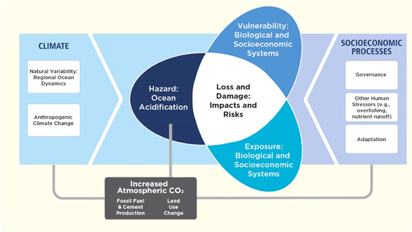
Figure 1. Framework adapted from IPCC (2012) to examine loss and damage, including both harm from observed impacts and projected risks from ocean acidification for illustrative regions.
Download figure:
Standard image High-resolution imageWe also draw upon existing literature and fisheries harvest databases maintained by the US National Oceanographic and Atmospheric Administration (NOAA) and the Food and Agriculture Organization of the United Nations (FAO) to identify biological systems of significant socioeconomic value. In doing so, we identify regions with initial indications of the types of human and biological systems that are exposed to ocean acidification and related climate stressors. These allow a first look at the potential adaptive capacity of the biological and socioeconomic systems to confront ocean acidification (figure 1).
3. Results
3.1. Atmospheric CO2 and global ocean pH
Total historical emissions from coal, oil, gas, and cement increase at a relatively low rate from the mid-1800s until the pace begins to increase rapidly in the mid-1900s (IPCC 2013). As expected, one of the most direct consequences of carbon emissions is the interaction with the carbon cycle, as measured by the growth rate in annual average atmospheric concentration of CO2, and after a year lag, the global surface ocean pH (see equation (1)). Accordingly, removing the annual emissions traced to the 88 largest industrial carbon producers from the production, refining, and end use of their products between 1880 and 2015 account for 60.8 (±4.4)% of the rise in atmospheric CO2 (supplementary information figure 5 and table 3). When emissions tied to these carbon producers are removed from 1965 to 2015, these account for 56.5 (±3.6)% of the rise in atmospheric CO2 over the 1880–2015 period (supplementary table 3). Uncertainty values, unless otherwise indicated, are based only on uncertainties from the fit of the simple global model that includes a range of sensitivity parameters and accounting for uncertainty arising from the lack of data on aerosol forcing traced to specific carbon producers (supplementary information). Other uncertainty sources are discussed at the end of this sub-section.
Model results show that, as a consequence, 55.3 (±2.0)% and 51.0 (±1.9)% of the decline in the surface ocean's pH between 1880 and 2015 can be traced to the 1880–2015 and 1965–2015 emissions, respectively, from these carbon producers (figure 2, supplementary table 4).
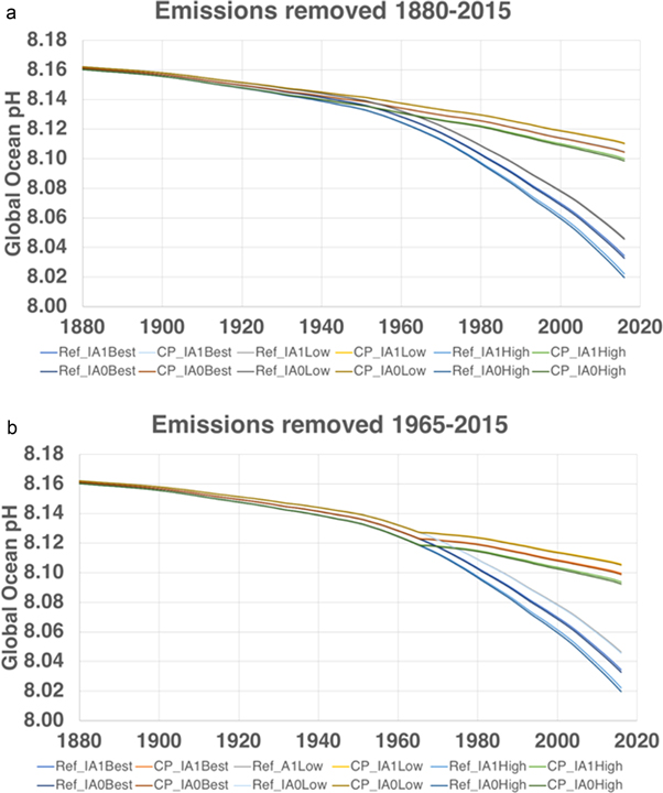
Figure 2. Calculated decrease in surface ocean pH over the historical time period (1880–2015) with natural and anthropogenic forcing and after emissions traced to the largest carbon producers were removed over ((a), 1880–2015), and ((b), 1965–2015). Abbreviations: Ref is the reference case natural and anthropogenic full forcing with carbon producers; CP is the reference case minus emissions tied to carbon producers over the years indicated; IA1 = full forcing including total historical fossil aerosols; IA0 = full forcing minus total historical fossil aerosols; Best, High, Low are parameters that correspond to values in supplementary information tables 1 and 2; see section 2.1.
Download figure:
Standard image High-resolution imageThe IPCC Fifth Assessment Report highlights the 0.1 unit decrease in surface ocean pH or an increase in hydrogen ion concentration by more than 26% since pre-industrial times (IPCC 2013). Our calculations find that the largest carbon producers contribute to more than half of that change. Emissions over 1880–2015 and 1965–2015 traced to the 20 largest investor-owned and majority state-owned carbon producers alone have contributed 25.0 (±0.8)% and 22.7 (±0.7)%, respectively, of the calculated decline in the surface ocean's pH between 1880 and 2015 (using forcing described in figure 3).
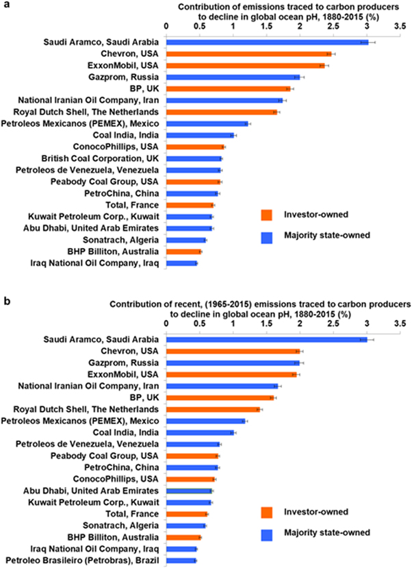
Figure 3. Contribution of the emissions traced to top 20 investor-owned and majority state-owned industrial carbon producers to the calculated decrease in surface ocean pH over the historical time period (1880–2015) after emissions traced to carbon producers' emissions were removed over ((a), 1880–2015), and ((b), 1965–2015) using best estimate parameters and full forcing including total historical fossil aerosols.
Download figure:
Standard image High-resolution imageThe relative contribution of atmospheric CO2 rise from fossil fuel and industrial emissions versus deforestation and land-use emissions is not fully resolved. Le Quere et al (2018) find that land-use and deforestation fluxes contribute ∼31% of cumulative historical CO2 emissions (1880–2017), with substantially larger uncertainties than fossil fuel emissions. This translates into uncertainties in the range of 10%–15% in attribution of fossil fuel emissions to changing surface ocean pH.
3.2. Regional acidification
Using the 3D ocean biogeochemical model to capture the regional variations in ocean acidification, we find that substantial surface pH declines occur in many regions (figures 1 and 2 and in the supplementary information). Elevated atmospheric CO2 is the predominant driver of the modeled surface seawater chemistry signals, which are also modulated by seawater thermodynamics, background upwelling patterns, and time-evolving ocean physics, surface warming and biogeochemistry. These findings are broadly consistent with previous studies (Feely et al 2009) where substantial surface pH declines occur across the temperate and polar ocean in both hemispheres, with the largest declines in the Arctic and western Antarctic Peninsula associated with reduced sea-ice cover. Similarly, the largest declines in surface aragonite saturation state occur over warm tropical waters. Temperature modulation of seawater carbonate thermodynamics via the background carbonate ion concentration and the inorganic carbon Revelle factor plays a fundamental role in the large-scale model patterns in Δ saturation (larger decline in warmer waters) and Δ pH (slightly larger decline in colder waters) (Δ refers to the difference between two time periods; Feely et al 2009, Fassbender et al 2018, Feely et al 2018).
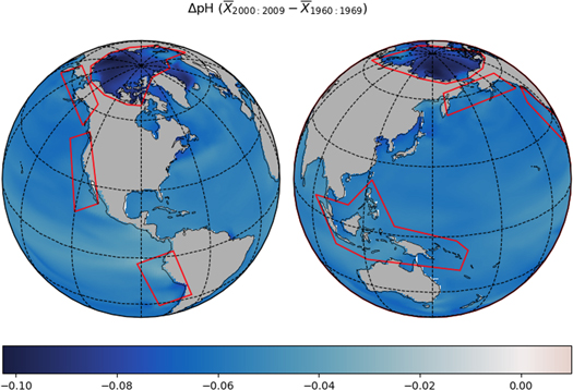
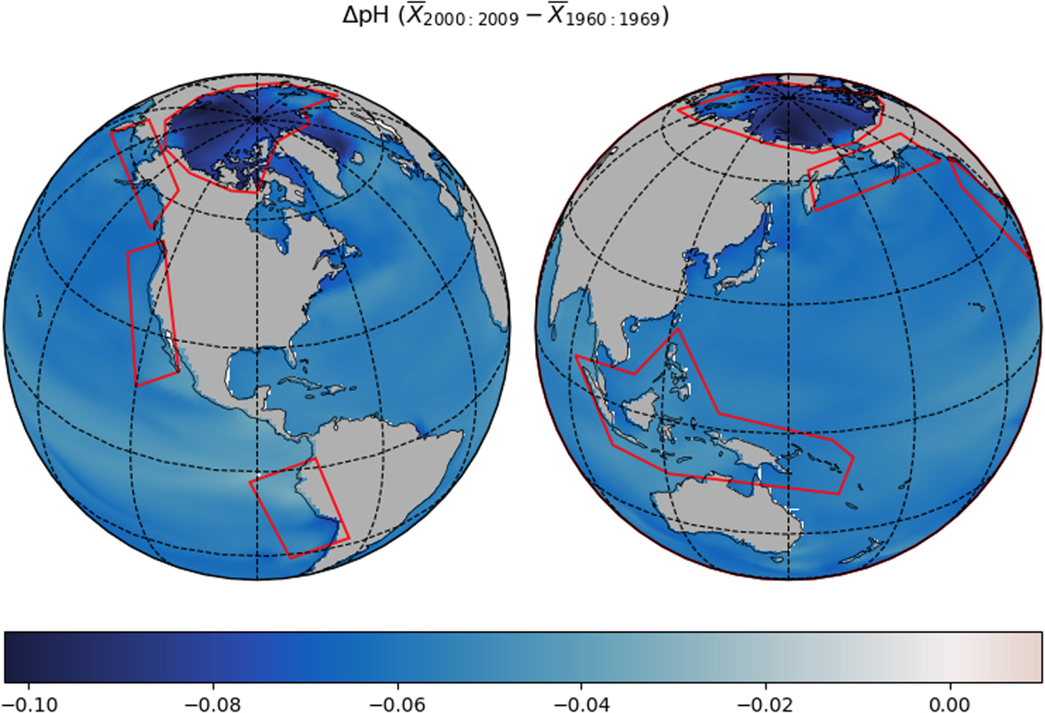
Figure 4. Modeled change in average surface ocean pH from 1960–1969 to 2000–2009. Red boxes demarcate the regions examined in detail in this study.
Download figure:
Standard image High-resolution image
Figure 5. Modeled change in regional surface ocean pH and aragonite saturation from 1850–1859 to 2000–2009 and from 1960–1969 to 2000–2009. Regions correspond to the red boxes in figure 4.
Download figure:
Standard image High-resolution image
Smaller-scale regional signals, however, are less robust across different ocean models and should be interpreted with caution. These include the localized saturation state declines for the most recent time-period off Japan and eastern North America (e.g. the Gulf of Maine) in CESM that occur as a result of latitudinal shifts in the location of western boundary currents.
The model was used to identify five regions where moderate-to-large surface seawater chemistry changes are co-occurring with substantial socio-economic dependence on vulnerable marine ecosystems: the Coral Triangle; the Bering Sea and Gulf of Alaska; the Peru Current; the Arctic Ocean; and the California Current (figures 4 and 5). Note that because of the relatively coarse resolution (∼1°) used in the global simulation, small-scale details of the spatial patterns in figure 4 may not fully capture narrow features, such as intense near-shore coastal upwelling. Variations in the overall regional patterns displayed in figure 5 are more robust.
Beyond the direct hazard of decreased surface ocean pH and aragonite saturation levels, each region contains at least one ocean dynamic that increases the effects of changes in global atmospheric CO2 levels (table 1; supplementary information). For example, the Gulf of Alaska's sensitivity to ocean acidification is increased by the upwelling of high-pCO2 waters that are undersaturated with aragonite (Evans et al 2013). Coastal upwelling also enhances the sensitivity to acidification in eastern boundary current systems off California and Peru (e.g. Hauri et al 2009), and some climate studies suggest that the intensity of eastern boundary current coastal upwelling may already be intensifying because of climate change (Sydeman et al 2014). We further identify other stressors stemming from anthropogenic climate change and other human activity that may exacerbate the effects of increasing atmospheric CO2 on ocean pH and aragonite saturation levels, such as tidewater glacial melt (Evans et al 2014) and pollution (Norman 2011) in the Gulf of Alaska.
These regions also contain biological systems that are vulnerable to ocean acidification (tables 1 and 2) and important to local human communities. The exposure of these important biological systems thus exposes communities to loss and damage from ocean acidification, now or in the near future (tables 1 and 2). Each ecosystem or human community has different vulnerabilities to current impacts and risks of further harms, because of its own composition, strengths, and weaknesses. For example, the Coral Triangle (the archipelago that includes Indonesia, Malaysia, the Philippines, Papua New Guinea, the Solomon Islands and Timor Leste) has the highest concentration of marine biodiversity in the world (Hoeksema 2007, Carpenter et al 2008). An estimated 76% of reef building coral species inhabit the region (Veron et al 2011). According to the International Union for Conservation of Nature (IUCN), the Coral Triangle contains the largest proportion of coral species categorized as Vulnerable and Near Threatened (Carpenter et al 2008). The marine biodiversity in this region and the food, livelihoods, and coastal protection that it affords supports more than 100 million people (Hoegh-Guldberg et al 2009). Consequently, communities within the Coral Triangle may be considered to be at relatively high risk of loss and damage due to ocean acidification coupled with other environmental threats to coral reef systems (Pendleton et al 2016). Communities in each region have substantial, yet differing, dependence on marine harvests and coastal industries. California and Peru Currents have large annual fisheries landings and/or a large number of jobs from aquaculture. The Coral Triangle has substantially sized fisheries that depend on coral reefs. Many residents of Coral Triangle nations depend on fisheries and aquaculture for livelihoods and subsistence (table 2).
Table 1. Components of risk of loss and damage from ocean acidification in five, illustrative regions of the world: The regional ocean dynamics amplifying exposure to global changes in atmospheric CO2 (stressors), the exposed biological system of importance and non-ocean acidification sources of biological vulnerability, and the socioeconomic systems exposed and the source of their vulnerability other than acidification from anthropogenic atmospheric CO2. Together with changes in surface ocean pH and aragonite saturation between 1850 and 2009 (climate-related hazards, figure 5), these elements result in the regions facing substantial loss and damage from ocean acidification. Anthropogenic, global ocean acidification and climate change resulting from human-caused increases in greenhouse gas emissions, and subsequently, atmospheric CO2 and methane levels, is the background condition for each region. Sources: (Harwell et al 2010, Norman 2011, Burke et al 2012, Asian Development Bank 2014, Mathis et al 2015b, Afflerbach et al 2017).
| Region | Anthropogenic climate change stressors | Natural stressors | Non-climatic, anthropogenic stressors | Biological system exposure and vulnerability | Socioeconomic system exposure and vulnerability | Loss and Damage—Impacts and Risks |
|---|---|---|---|---|---|---|
| Coral Triangle (Malaysia to Solomon Islands to Philippines) | Rising temperatures | Land- and marine-based pollution, overfishing, destructive fishing, coastal development | Highest concentration of marine biodiversity in the world. Coral reefs here are already experiencing widespread bleaching due to heat and disease | Surrounding countries depend on coral reefs for tourism and other livelihoods, coastal protection, and food. Nations have developing economies. Poverty and hunger are also problems | Risk of loss of marine biodiversity; poverty and hunger exacerbation, lost wages; Increased exposure to storms | |
| Bering Sea & Gulf of Alaska | Rising temperatures, sea ice and glacial melt | Biological production, riverine input, upwelling | UV radiation, land-based pollution, fishing, oil spills, shipping, acoustic pollution, point-source and nonpoint source pollution | Source of 40% of US fish catch, including crab and groundfish species. Attentive fisheries management is maintaining high harvest levels | Alaskan commercial and subsistence fishing communities, including Native Alaskan communities, have high economic and nutritional dependence and low livelihood alternatives | Risk of losses to important fisheries and increased food insecurity; loss of livelihoods, and economic damages |
| Peru Current | Rising temperatures, climate-altered upwelling | Upwelling | Fishing | Highly productive anchovy and sardine fisheries (alternating) | Large commercial fisheries are dependent on catch from the Peru Current | Risk of losses to important fisheries and increased food insecurity; loss of livelihoods and economic damages |
| Arctic Ocean | Rising temperatures, glacial and sea ice melt | Riverine input, seasonal upwelling | UV radiation, shipping, oil spills, acoustic pollution | Short food web with low species diversity for several marine ecosystem niches | Subsistence fishing | Risk of loss of marine biodiversity; increased food insecurity |
| California Current | Rising temperatures, oxygen loss, changes to fresh water runoff, climate-altered upwelling | Upwelling, atmospheric oscillations like ENSO, PDO | Shipping, heavy coastal development, altered fresh water use, fishing | Highly diverse marine ecosystem, with unique micro-environments. | Large commercial fisheries dependent on catch from California Current. Broad economic diversity in coastal communities with many livelihood alternatives | Risk of loss of marine biodiversity; loss of livelihoods; economic damages |
Table 2. Examples of biological and socioeconomic systems facing loss and damage from ocean acidification. Communities in each region have substantial, yet differing, dependence on marine harvests and coastal industries. California and Peru Currents have large annual fisheries landings and/or a large number of jobs from aquaculture. The Coral Triangle has substantially sized fisheries that depend on coral reefs. Many residents of Coral Triangle nations depend on fisheries and aquaculture for livelihoods and subsistence.
| Region | Sub-region | Quantity of fisheries landings (tonnes, 2016 value or estimate) | # of jobs from fishing, without imports | # of jobs from aquaculture | Population in coastal zone | Value of fisheries attributed to coral reefs ($, 2007) | % of population dependent on fisheries and aquaculture |
|---|---|---|---|---|---|---|---|
| Bering Sea/Gulf of Alaska | Alaska | 2533 750a | 53 131c | N/A | N/A | N/A | N/A |
| California Current | California | 80 016a | 9105c | 1266g | 25 520 252h | N/A | N/A |
| Oregon | 95 022a | 11 347c | 107g | 653 112h | N/A | N/A | |
| Washington | 250 322a | 22 887c | 204g | 4615 192h | N/A | N/A | |
| Peru Current | Peru | 3831 131b | 67 600d | 10 780d | N/A | N/A | N/A |
| Chile | 2878 440b | 88 900e | 1300e | N/A | N/A | N/A | |
| Coral Triangle | Indonesia | 19 328 054b | 2641 566f | 2493 193h | 64 783 600i | 1528 613 328i | 8.9i |
| Malaysia | 1882 562b | 125 632f | N/A | 8928 000i | 439 911 551i | 1.8i | |
| Philippines | 3769 394b | 1388 173f | 226 195h | 43 346 502i | 932 886 834i | 7.0i | |
| Papua New Guinea | 299 759b | 120 000f | N/A | 1460 040i | 8117 310i | 9.5i | |
| Solomon Islands | 77 025b | 5114f | N/A | 433 331i | 67 225 540i | 5.0i | |
| Timor Leste | 4706b | 7600f | N/A | 551 166i | 23 270i | 3.7i |
aFisheries of the US 2016. https://fisheries.noaa.gov/webdam/download/62276710 bFAO Global Production Statistics, queried 27 August 2018; 2016 values/estimates. http://fao.org/fishery/statistics/global-production/en cFisheries Economics of the US 2015. https://fisheries.noaa.gov/feature-story/fisheries-economics-united-states-2015 d2014 values from http://fao.org/fishery/facp/PER/es e http://fao.org/fishery/facp/CHL/es. fCapture fisheries employment (primary sector). Economics of Fisheries and Aquculture in the Coral Triangle. 2014. Asian Development Bank. https://adb.org/sites/default/files/publication/42411/economics-fisheries-aquaculture-coral-triangle.pdf. g2010 values from The Economic Impacts of Shellfish Aquaculture in Washington, Oregon and California. Northern Economics. 2013. hTotal population of coastal counties in 2010. NOAA. https://aamboceanservice.blob.core.windows.net/oceanservice-prod/facts/coastal-population-report.pdf. iEconomics of Fisheries and Aquaculture in the Coral Triangle. 2014. Asian Development Bank.
4. Discussion and conclusion
Over both historical (1880–2015) and recent (1965–2015) time periods, more than half of the global surface ocean acidification is attributable to the CO2 emissions traced to the extraction, refining and combustion of fossil fuels and manufacturing of cement from the 88 largest carbon producers. Over equivalent time periods, the proportion of global acidification attributed to these carbon producers is similar, albeit slightly less than, the proportion of atmospheric CO2 attributable to them. This is because there is a close relationship (equation (1)) between atmospheric CO2 levels and global surface ocean pH.
Of these 88 major carbon producers, 48 are investor-owned fossil fuel companies whose climate responsibilities are the focus of growing policy, legal and societal scrutiny. Emissions from majority state-owned and nationalized companies fall within the primary responsibilities of nation-states. Emissions traced to extraction, refining, marketing, and combustion of fossil fuels by these 48 investor-owned companies between 1965 and 2015 account for 15.5(±0.6)% of global ocean acidification over the total historical period. Historical evidence suggests that by the mid-1960s, fossil fuel companies were aware that unabated emissions from the continued use of their products posed substantial climate risks (Franta 2018). The ethical philosopher Henry Shue (2017) argues that, from this point on, companies had a responsibility to 'modify or substitute in order to stop contributing to harm. This is not complicated or controversial and is a widely shared social judgment.'
Global data provide a useful starting point for quantifying the contribution of the largest industrial carbon producers to ocean acidification, and in turn, considering what share of responsibility they may hold for its societal impacts. However, the non-uniform distribution of ocean acidification across marine regions suggests value in exploring regional-to-local impacts and risks, as some regions may face greater loss and damage from ocean acidification than others. In contrast to those previous studies that emphasized global and basin-scale changes, the regional analysis of the 3D ocean carbon presented here is guided by recent research that identifies regional components of risk of loss and damage from ocean acidification (table 1). This synergy highlights paths forward for coupled natural and social science research. Further, such regional analyses may also help draw attention to synergies among multiple drivers of loss and damage from carbon producer-traced emissions, such as increased frequency and intensity of ocean heatwaves that induce coral bleaching events where coral recovery may be hampered by more acidic water (Hoegh-Guldberg et al 2017).
Regional-scale variables related to fisheries harvest may provide first-order proxies for socioeconomic vulnerability to ocean acidification. The Bering Sea and Gulf of Alaska, California Current, Coral Triangle, and Peru Current have substantial, high-value fisheries and fisheries-related jobs (tables 1 and 2). For example, the US states within the California Current region reported fisheries landings of 425 360 tonnes in 2016, supporting more than 40 000 jobs (table 2). The California Current also supports a coastal aquaculture system upon which more than 1500 jobs directly depend. In 2010, the shellfish aquaculture industry, a sector that is under direct threat from ocean acidification (Barton et al 2015), generated an estimated $90.3 million of revenue in Washington State, $25.8 million in California, and $9.3 million in Oregon (Northern Economics 2013). Across the three states, this industry supported more than 1400 jobs during that time (Northern Economics 2013), often in rural areas where employment can be scarce. Within the Coral Triangle, the fisheries associated with the region's coral reefs in the region are worth nearly $3 billion a year (2007 figures, table 2). The fisheries from the Peru Current yielded 6.7 million tonnes of landings in 2016 and supported more than 156 000 jobs.
Importantly, such economic proxies leave out key impacts on ecosystems and human communities facing loss and damage from ocean acidification. For example, the Arctic Ocean, which is experiencing rapid decreases in ocean pH, does not yet have significant economically valuable fisheries. Describing the likely impacts of ocean acidification on its ecosystems remains primarily in the qualitative realm (e.g. Mathis et al 2015a, AMAP 2018, etc).
Although variables related to fisheries harvest and coral reef coverage provide coarse proxies for ecosystem services and socioeconomic dependence on marine resources, important nuance is lost, somewhat limiting the socioeconomic conclusions that can be drawn. Furthermore, as we are not able to quantify the interaction between all ocean changes stemming from anthropogenic carbon emissions, we likely underestimate the full loss and damage to marine biodiversity and communities stemming from emissions traced to major industrial carbon producers. For example, ecosystem models incorporating the effects of ocean acidification and warming in the Puget Sound region show that different species and ecological communities experience varying levels of impacts under an acidifying ocean, because any predator/prey relationship changes caused by ocean change are also affected by behavior, fishing pressure, habitat availability, and more (e.g. Marshall et al 2017). Similarly, simply projecting estimated changes in coral reef coverage or quantitative assessments of fisheries harvests also underestimate the social-ecological changes relevant for benefits to humans beyond economic revenue. Factors including cultural importance, livelihoods, changing locations of dominant ports, social opportunities to benefit from marine resources, and more could be substantially altered and currently run the risk of being dramatically undervalued.
By focusing solely on surface ocean pH (and carbonate mineral saturation state), this paper provides a conservative basis for assessing the contribution of emissions traced to major carbon producers to marine loss and damage. The impacts of acidification on marine ecosystems and human communities dependent upon them can be amplified by ocean warming and other climate-change stressors; further modeling of these compound stressors could quantify the contribution of carbon producer-traced emissions to these impacts.
Lags in the carbon cycle, such as the centuries-long lifetime of CO2 within the ocean-atmosphere system and timescales of the ocean circulation system, mean that the impacts stemming from historical emissions have not fully been expressed; future loss and damage may in part be attributable to past emissions. But the extent and severity of future harms of ocean acidification and climate change on marine species and ecosystems, and the human communities dependent upon them, will be largely determined by the future course of further carbon emissions. In high-value fisheries such as those harvesting Alaska red king crab and Atlantic sea scallop, decreases associated with ocean acidification are projected to become apparent in the next 20–30 years, when effects exceed natural variation (Punt et al 2014, Cooley et al 2015, Rheuban et al 2018). Further acidification is projected to alter temperate ecosystems' fishery yield and overall structure (Busch et al 2013, Fay et al 2017).
The results of this analysis contribute to a growing body of scientific literature that attributes specific climate impacts and damages to non-nation state entities. Furthermore, we take previous work that ties carbon emissions to the largest industrial carbon producers and attributes climate impacts to those emissions a step further, by beginning to demonstrate the potential associated losses and damages from ocean acidification. The regions examined here are disproportionately vulnerable to impacts of greenhouse gas emissions to date—a large portion of which originate from the world's largest carbon producers (Heede 2014, Ekwurzel et al 2017). This work also points to a new avenue of research—one that quantifies the ties between regional changes such as changes in surface ocean pH detected here to individual carbon sources. Such work would continue to advance considerations of responsibility for the changes, impacts, and risks and could be extended into a variety of climate domains—from changes in temperature to sea level rise.
Acknowledgments
The approach of using equation (1) benefited from discussions with Myles R Allen (University of Oxford) and Inez Fung (University of California, Berkeley). M W Dalton provided insights for the incorporation of the updated carbon producers data. Chloe Ames provided support for references. S Doney acknowledges support from the US National Science Foundation and the University of Virginia Environmental Resilience Institute. R Licker, B Ekwurzel and P C Frumhoff acknowledge the support of the Grantham Foundation for the Protection of the Environment, Wallace Global Fund, and Rockefeller Family Fund to the Union of Concerned Scientists. R Heede gratefully acknowledges the financial support of Wallace Global Fund, Rockefeller Brothers Fund, and Union of Concerned Scientists. We thank two anonymous reviewers for their helpful comments, which greatly improved our manuscript.
Data availability statement
Any data that support the findings of this study are included within the article.