A Comparison of Forest Tree Crown Delineation from Unmanned Aerial Imagery Using Canopy Height Models vs. Spectral Lightness


Department of Natural Resources & the Environment, University of New Hampshire, 56 College Rd, Durham, NH 03824, USA
*
Author to whom correspondence should be addressed.
Forests 2020, 11(6), 605; https://doi.org/10.3390/f11060605
Submission received: 2 May 2020
/
Revised: 22 May 2020
/
Accepted: 23 May 2020
/
Published: 26 May 2020
(This article belongs to the Special Issue Mapping and Monitoring Forest Cover)
Abstract
:Improvements in computer vision combined with current structure-from-motion photogrammetric methods (SfM) have provided users with the ability to generate very high resolution structural (3D) and spectral data of the forest from imagery collected by unmanned aerial systems (UAS). The products derived by this process are capable of assessing and measuring forest structure at the individual tree level for a significantly lower cost compared to traditional sources such as LiDAR, satellite, or aerial imagery. Locating and delineating individual tree crowns is a common use of remotely sensed data and can be accomplished using either UAS-based structural or spectral data. However, no study has extensively compared these products for this purpose, nor have they been compared under varying spatial resolution, tree crown sizes, or general forest stand type. This research compared the accuracy of individual tree crown segmentation using two UAS-based products, canopy height models (CHM) and spectral lightness information obtained from natural color orthomosaics, using maker-controlled watershed segmentation. The results show that single tree crowns segmented using the spectral lightness were more accurate compared to a CHM approach. The optimal spatial resolution for using lightness information and CHM were found to be 30 and 75 cm, respectively. In addition, the size of tree crowns being segmented also had an impact on the optimal resolution. The density of the forest type, whether predominately deciduous or coniferous, was not found to have an impact on the accuracy of the segmentation.
1. Introduction
Forests not only mitigate global climate change, sustain biodiversity, and prevent soil erosion; they also provide raw materials and resources such as timber, fresh food, and herbal medicines [1,2,3]. Maintaining the diversity of these products and services involves the development and implementation of forest management practices, which requires detailed forest inventory information at varying scales, such as stand-level basal area and diameter at breast height (DBH), and/or crown size and tree height at the single tree level [4,5,6].
The conventional way to gather this forest inventory information is to carry out periodic field surveys based on statistical sampling [7,8]. Nevertheless, the high cost in time and expense, as well as the difficulties in accessing specific sampling locations, make it an inefficient and often impractical approach [9,10]. Furthermore, data collected from in situ measurements, as shown in recent studies, is not as reliable due to many uncertainties such as sampling and observational errors [11,12,13]. Over the last few years, unmanned aerial systems (UAS), carrying a variety of sensors ranging from standard consumer-grade cameras to more expensive and complex multispectral or light detection and ranging (LiDAR) sensors, have offered a potential solution to extend or replace field observations because of its ability to provide higher spatial resolution imagery and/or 3D data to quantify structural and compositional information at the single tree level [10]. This ability, combined with the tremendous progress in the techniques of digital image processing, has led to a sharp increase of these applications to precision forestry [14,15,16].
Individual tree locations and their crowns are the building blocks on which other parameters such as tree height, diameter at breast height (DBH), or biomass are estimated [17,18,19]. Treetops mark the tree locations and typical algorithms to detect them include local maximum filtering, image binarization, multiscale analysis, and template matching [12]. Methods to delineate tree crowns consist of three categories: valley following, watershed segmentation, and region growing [9,12]. The watershed algorithm, because of its intuitive and computationally efficient features, is one of the most commonly used segmentation algorithms for tree crown delineation. The algorithm metaphorically regards the whole grayscale image or model as a topographic surface where the watershed lines are the boundaries of trees [20,21]. However, due to its high sensitivity to noise and spectral variation, it is prone to oversegmentation, a situation where multiple segments fall within what should be a single tree crown [22]. Many improved watershed algorithms such as edge-embedded, marker-controlled, or multiscale approaches were developed to overcome this problem [23,24]. The marker-controlled watershed algorithm, which adds marker regions or points corresponding to one segmented object, was shown to be robust and flexible [20,25,26]. Many studies successfully applied a marker-controlled watershed to delineate tree crowns and achieved accuracies over 85% [22,27].
The data for detecting treetops or segmenting individual tree crowns could be derived either photogrammetrically or from LiDAR [12,28,29]. Digital photogrammetry is favored by many researchers to calculate forest inventory metrics because of its ability to provide orthometrically corrected imagery (orthoimagery) in addition to 3D point clouds for a much lower price compared to a LiDAR system. The point clouds derived from photogrammetry are extracted from stereo images based on structure-from-motion (SfM) and multiview stereopsis (MVS) techniques [30,31,32]. However, unlike the LiDAR-based point cloud, because of its inability to penetrate the foliage to achieve the ground information, it can only generate a digital surface model (DSM) for dense forests [33]. An external digital terrain model (DTM) is usually needed to create the canopy height model (CHM) representing the height of objects above the ground. Either the orthoimagery or CHM can then be used for tree segmentation [28,34]. Most research developed algorithms assuming that tree canopies possess mountainous shape, where treetops are the locally brightest in the image or the locally highest in the CHM data, while tree edges are darker or lower in elevation [12,35]. Very little research has examined and compared the accuracies of tree crowns segmented from UAS and photogrammetrically-based imagery and CHMs, especially within dense coniferous and deciduous forest stands.
Data that are photogrammetrically generated are of exceptionally high spatial resolution (e.g., pixel size of a few centimeters) but often provide too much detail. For example, tree branches and gaps between leaves increases the spectral or height variation within the tree crown, adding to the uncertainty for tree crown segmentation [22,36]. Upscaling, decreasing the spatial resolution of the original data, is one way to reduce this noise, but it can also weaken the distinction between tree crowns [12,22]. Additionally, canopies of different sizes may have varying degrees of sensitivity to the chosen spatial resolution. Intuitively, as the spatial resolution decreases, the segmentation accuracy of the larger crowns may increase because potential noise within the crown is reduced. In contrast, the accuracy of smaller crowns declines because they may disappear in coarser images [12]. Therefore, a tradeoff exists between the tree size and spatial resolution; thus, it would benefit users to find the best spatial resolution for specific tree crown sizes.
The objectives of this study are to (1) compare the accuracies of individual tree crowns delineated from UAS-based CHMs and natural color orthoimagery using maker-controlled watershed segmentation, (2) provide insight into how accuracies change with spatial resolution, crown size, and forest type (coniferous or deciduous), and (3) facilitate the consideration of choosing the right data and scale for individual tree delineation in the future.
2. Data and Methodology
2.1. Study Site and Data Collection
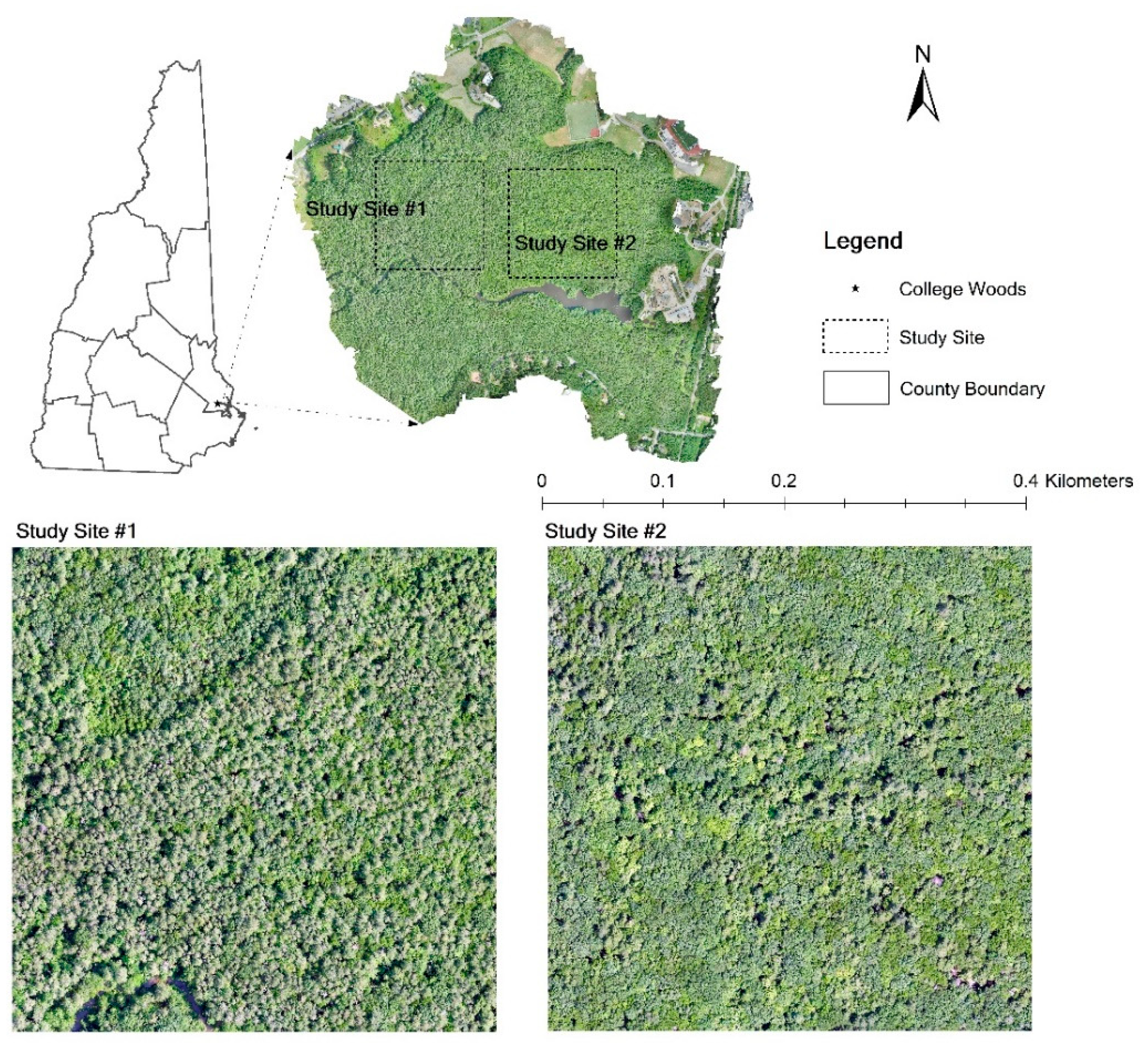
This research took place within the College Woods Natural Area (CWNA, Figure 1), 70°56′51.339″ W and 43°8′7.935′ N, in Durham, NH, USA. The CWNA is owned and managed by the University of New Hampshire. The annual average precipitation for the region is 119.38 cm with a yearly average temperature of 8.84 °C. Two soil types, Buxton and Hollis–Charlton, dominate this area. White pine (Pinus strobus), eastern hemlock (Tsuga canadensis), American beech (Fagus grandifolia), and several species of oak (Quercus spp.) are the primary tree species/genera. Two study sites, each covering a 400 × 400 m area, were chosen within the CWNA. Both study sites are a mixed forest type; however, the coniferous tree species are most prevalent in study site #1, while the deciduous tree species are dominant in study site #2.
The raw UAS images were collected on 11 July 2018, with a fixed-winged SenseFly eBee Plus carrying a SODA (sensor optimized for digital acquisition) camera that captures natural color imagery. The flight was 120 m above the ground with a forward and side overlap of 85%. A total of 1961 photos, covering all of the CWNA, were collected.
2.2. Data Preprocessing
The first step of preprocessing was to create an orthomosaic and DSM from the UAS imagery. All the raw images were processed with Sensefly’s Flight Data Manager built into the eMotion software [37]. First, the geotags for all the images collected during the mission were extracted from the mission flight log and Post-Processed Kinematic (PPK) processed using a nearby Continuously Operating Reference Station (CORS) (site ID: NHUN). The images were then geotagged with the PPK corrected positions. Due to the density of the canopy cover, ground control points could not be collected across the CWNA. The images were further processed by Agisoft Metashape Pro (v.1.6.2) [38] to create a natural orthomosaic and DSM. The Agisoft workflow comprises five basic steps: align photos, build dense cloud, build mesh, build digital elevation model, and build orthomosaic [39]. We followed the suggestions provided by [40] to set the parameters for data processing. The spatial resolution of the orthomosaic and DSM was 2.31 and 12.10 cm, respectively.
The second step was to create a series of data sets with different spatial resolutions from the orthomosaic and CHM to test the effects of spatial resolution. The orthomosaic was converted from an RGB model into an HSL model, where the lightness band (L) represents pixel brightness. The lightness band is widely utilized for object segmentation [41,42]. The CHM model was created by subtracting a DTM from the UAS-based DSM. The DTM was made from LiDAR data collected for coastal New Hampshire in the winter and spring of 2011, and downloaded from the GRANIT LiDAR distribution site [43]. The 2-meter gridded raster DTM files, generated from ground-classified LiDAR returns, were provided as part of the project deliverables. Based on the size and land-use history of two study sites, the age of the DTM relative to the UAS missions would introduce little, if any, error. The DTM was reprojected to match the projection, coordinate system, and horizontal and vertical datum of the DSM. A series of datasets with different spatial resolutions were created by resampling the lightness band and CHM using cubic convolution in ArcGIS Pro 2.4.2 [44]. For the lightness band, the resampling started at 2 cm and was incrementally increased by 2 cm until a resolution of 100 cm was reached, resulting in 50 lightness datasets. The same process was performed on the CHM; however, the initial resolution was 12 cm, resulting in 44 CHMs.
2.3. Reference Tree Crown Data Collection
The reference data (i.e., individual reference tree crowns) were randomly collected from each study site and then manually interpreted by combining the natural color orthomosaic and CHM data. The workflow follows. First, 800 random sampling points were generated over each study site. Then, a trained undergraduate student manually digitized a tree if a point fell within the tree’s crown. If more than two points were situated within the same tree crown, only one tree crown was counted in. Any point that hit the background (not a tree) was removed. However, the edges of the canopy are highly curved, making digitizing work extremely arduous. In order to reduce the workload without losing the accuracy of reference data, an extremely oversegmented result was created by applying the multiresolution segmentation algorithm in eCognition 9.5.1 [45]. The scale, compactness, and shape parameters for the algorithm were set to 40, 0.5, and 0.5, respectively. Finally, the interpreter digitized the tree crown by merging the crowns’ oversegmented polygons into a single crown polygon. A few polygons may have still needed a splitting operation before merging, but this workflow improved the processing of delineating the reference data.
Another experienced researcher further examined the interpreted result, and all controversial objects were removed after discussion. The final reference tree crown polygons for a study site were divided into three groups, large, medium, and small trees, based on the crown area using natural division. For study site #1, the criteria of separation were: large (≥42.06 m2), medium (18.42–42.06 m2), and small (<18.42 m2). For study site #2, the criteria of separation were: large (≥51.20 m2), medium (21.74–51.20 m2), and small (<21.74 m2). The sample size in each group was uneven. To make all groups comparable, we randomly resampled all other groups without replacement using a sample size based on the group with the least number of samples across both study sites. That group was the large trees in Site #1 with only 174 reference trees.
2.4. Treetops Detection
This research applied a local maximum filter to detect the treetops which is highly dependent on crown size [46]. The window size was determined by calculating the average size of the tree crowns in the reference samples. The window size was set to 4.58 and 4.51 m for study site #1 and #2, respectively.
2.5. Marker-Controlled Watershed Segmentation
The watershed algorithm is a classical algorithm for segmentation, which was developed from mathematical morphology [47]. The marker-controlled watershed algorithm requires two inputs: (1) a gray scale image to represent the “topography” or highs and lows of the area, and (2) the point locations (i.e., markers) that define either local minimums or maximums within the gray scale image [48]. When the markers represent local minimums, the algorithm delineates a polygon around each marker containing higher gradient (i.e., spectrally brighter or topographically higher) pixels than that of the marker. In this research, local maximums representing treetops were used as the markers, inverting the processes so the delineated areas represent a decreasing gradient of values around the treetop. The area delineated around the marker in this case was assumed to represent that tree’s crown. The markers act as seed locations for the algorithm and, unlike traditional watershed segmentation, restricts the creation of basins to just those markers. This creates a one-to-one relationship between markers and segments or trees and crowns. Details of the marker-controlled watershed algorithm can be found in [20,49,50].
A Sobel filter, a widely used algorithm, was applied to each dataset to calculate gradients [51]. The marker-controlled watershed segmentation was applied to all the lightness bands and CHMs using scikit-image, an open source image processing library for the Python programming language [52]. It is worth noting that during the workflow, smoothing filters such as the Gaussian filter were not applied across the data to reduce noise because these filters are regarded as having a similar effect as reducing the spatial resolution. The combined operations would weaken the purpose of this research to explore the best scale for segmentation.
2.6. Accuracy Assessment
The accuracy assessment for segmentation is different from the one for traditional thematic classification [53]. The purpose of individual tree crown delineation is to represent each crown with a single polygon [12]. Therefore, before calculating the accuracy measures for each reference polygon, the best-matching segment from each segmentation result must be chosen to build a one-to-one relationship. The overlap index (OI) proposed by [54] was utilized in this research to find the single best candidate for each reference polygon.
In Equation (1), represents ith reference polygon and represents the jth candidate segmented polygon that intersects with . The symbol represents the intersection of and . ranges from 0 to 1, where a higher value indicates a better match.
This research employed oversegmentation accuracy (), undersegmentation accuracy (), and quality rate () to quantitatively validate the segmentation results [55,56].
In Equations (2) and (3), the indicates the best corresponding candidate. The sampling size is represented by . A higher or means greater accuracy. The proposed by [57] defines the accuracy between a reference polygon and its candidate by combining the overlapped and union region. It also considers the geometrical similarity. If a segmented object entirely coincides with its reference object, the reaches the minimum [56].
In Equation (4), the denotes a union. Higher indicates a less accurate segmentation.
3. Results
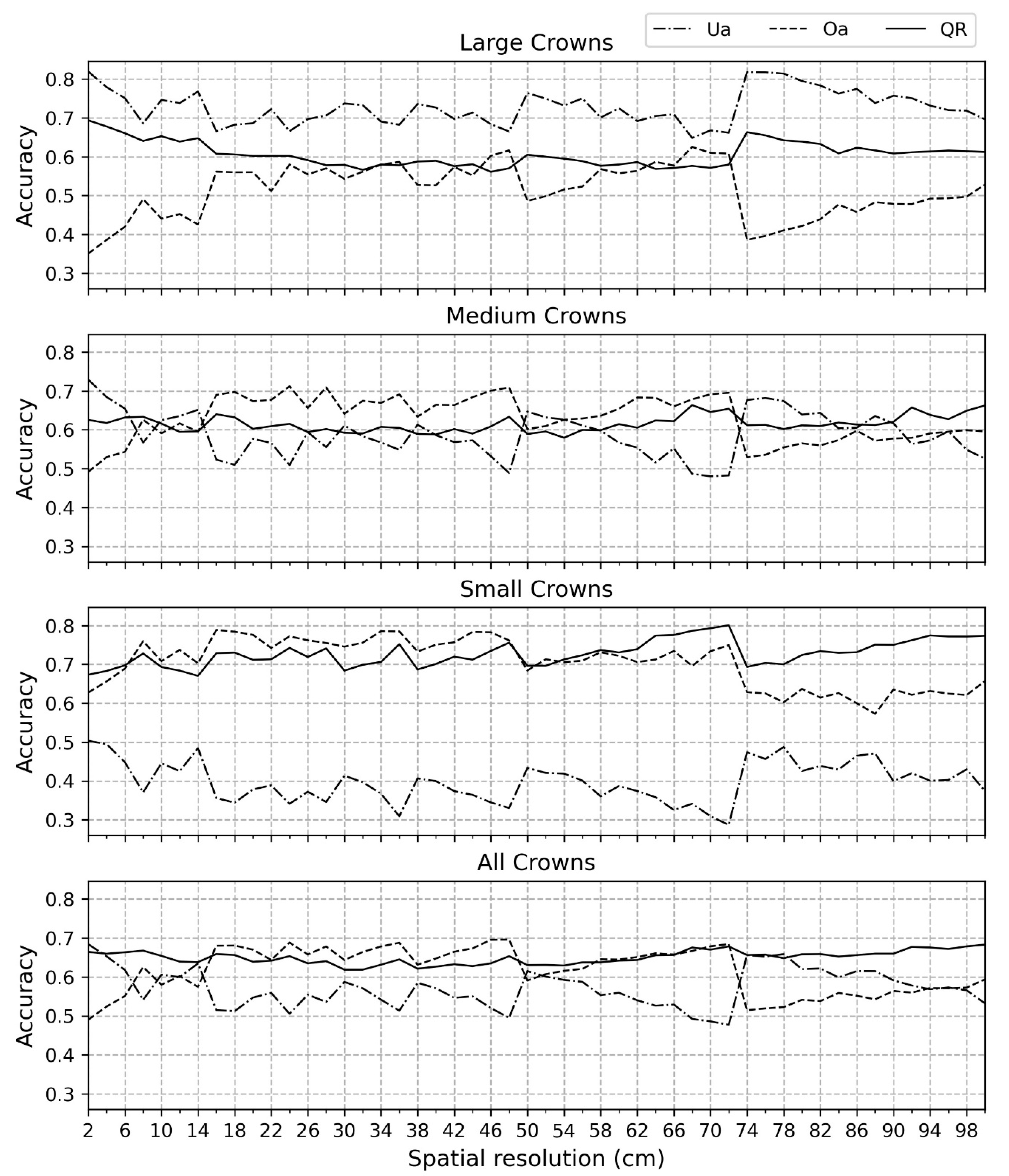
Figure 2 presents the Oa, Ua, and QR of all segmentations using the lightness band as the data source for study site #1. The accuracies are displayed for four groups: large, medium, small, and all crowns, as follows:
- (1)
- For large crowns, the Ua is higher than the Oa. Overall, the gap between Ua and Oa is narrower when the spatial resolution reaches between 16 and 72 cm. The Ua shows a downward trend while the Oa demonstrates an upward trend before the spatial resolution approaches 74 cm. Both the lines of Ua and Oa become stable when the spatial resolution is between 16 and 48 cm. The highest Ua is approximately 0.81 when the spatial resolution is 2 cm. The Oa reaches a maximum value of 0.62 when spatial resolution is 68 cm. The QR shows a general downward trend before the spatial resolution of 74 cm. The QR lies under 0.6 for spatial resolutions between 26 and 48 cm, and between 58 and 72 cm. As indicated by the minimum of QR, the best segmentation is achieved when the spatial resolution is 46 cm.
- (2)
- The lines of Oa and Ua for medium crowns intertwine, and the gap between them becomes narrower in contrast to the one in the large group. It results in a stable QR around 0.60. The lowest QR appears when spatial resolution is 54 cm.
- (3)
- The three accuracy measures for the small group are quite different. The line for Oa is much higher than the one for Ua. The gap between them becomes narrower after the spatial resolution reaches 74 cm. All Ua values are under 0.50. Most QR values are higher than 0.70, which is higher than the ones in either the large or medium groups.
- (4)
- Both the shape and values of Oa and Ua for all crowns parallel the medium crowns. The QR value varies between 0.60 and 0.70. The relative lower QR values appear when the spatial resolution lies between 30 and 62 cm.
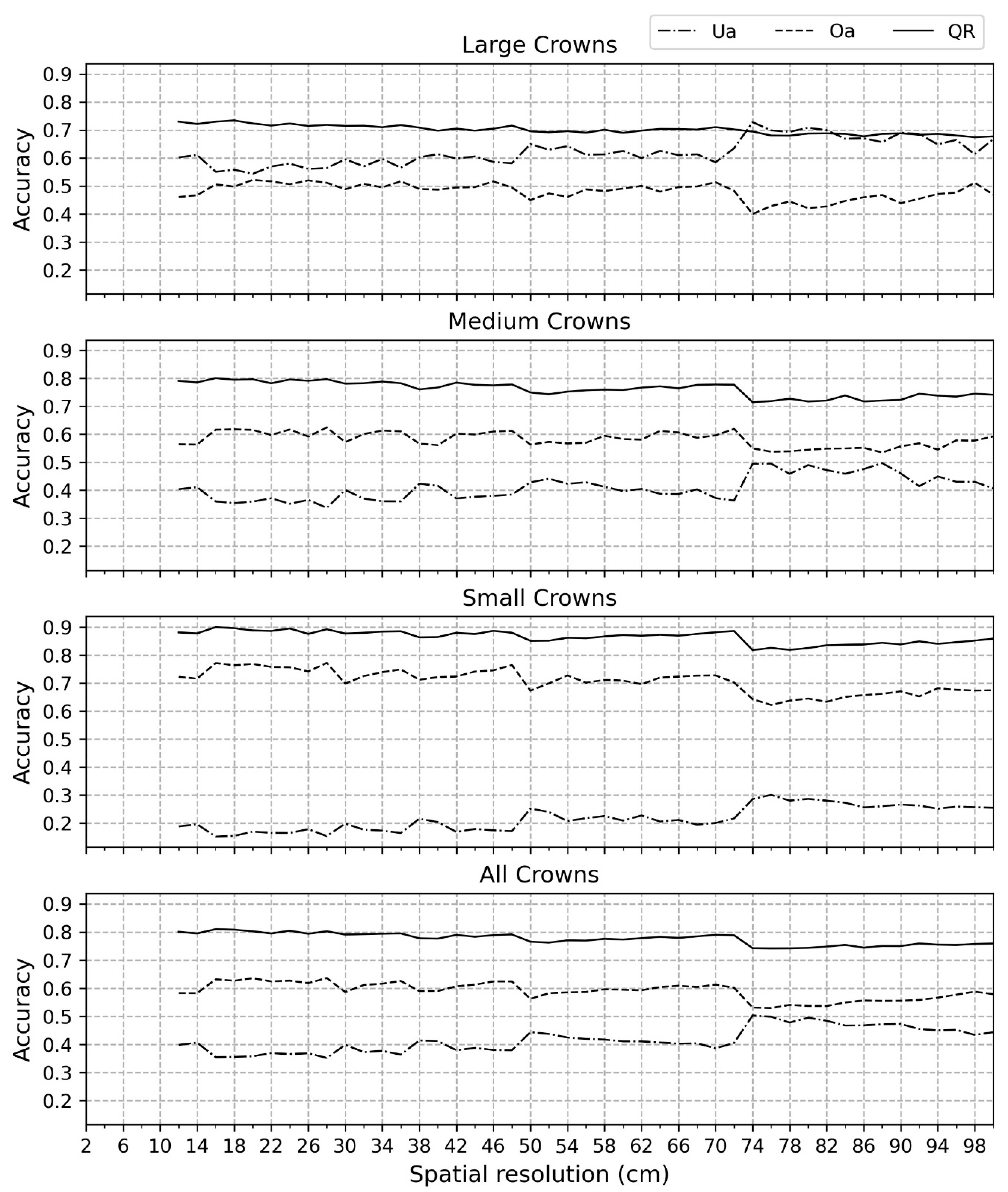
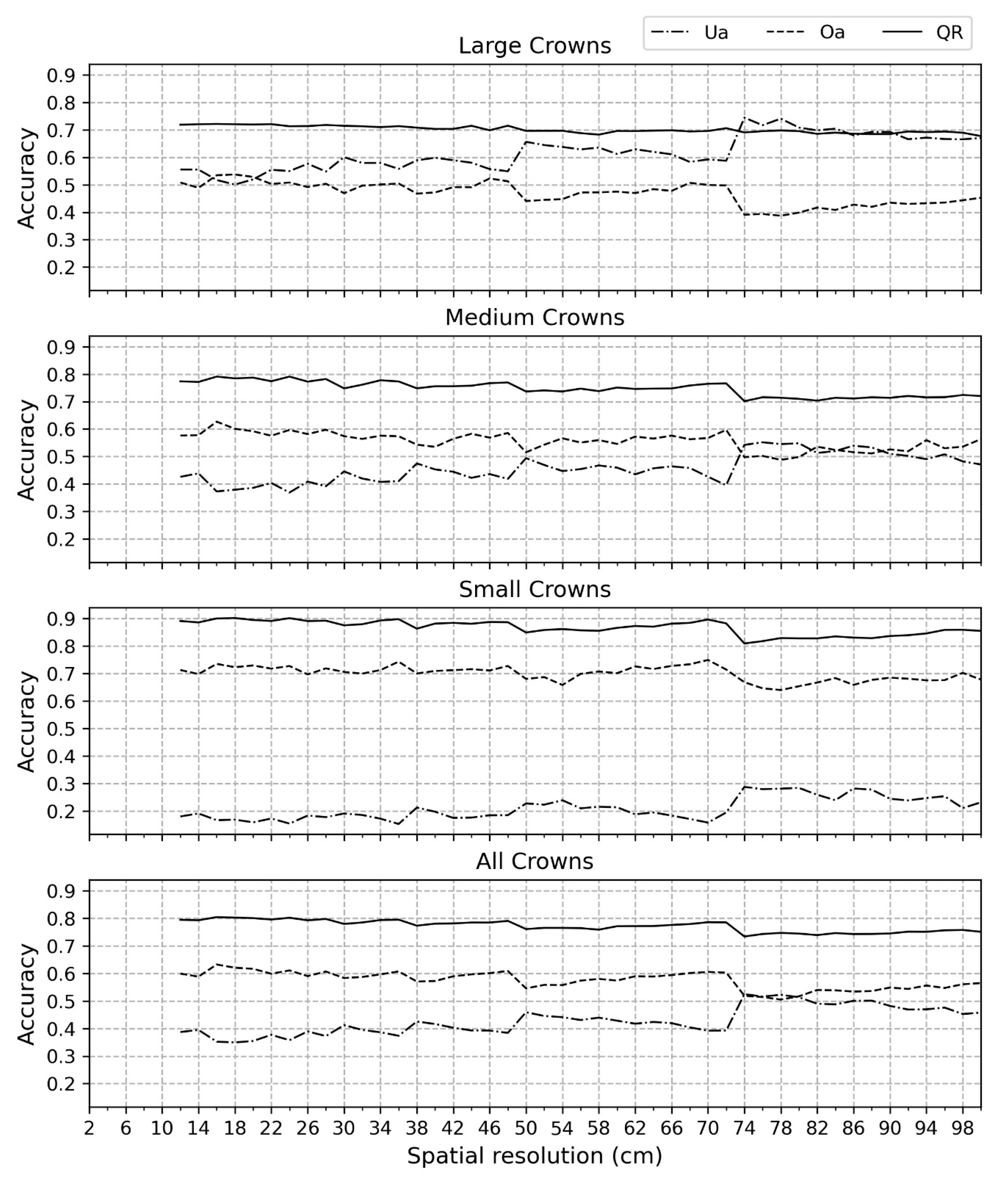
Figure 3 presents the accuracies after segmenting the CHM and exhibits a clear difference from Figure 2. First, the lines of Oa, Ua, and QR are highly stable for all crown sizes. Most values of Ua and Oa are lower than the ones in Figure 2, resulting in higher QR values. Second, within each group, the line of Oa is higher than the Ua except in the case of large crowns. The Ua reduces, and the Oa increases as the crown size grows. According to QR, the best spatial resolution for segmentation is 86, 78, 74, and 76 cm for the large, medium, small, and all groups, respectively.
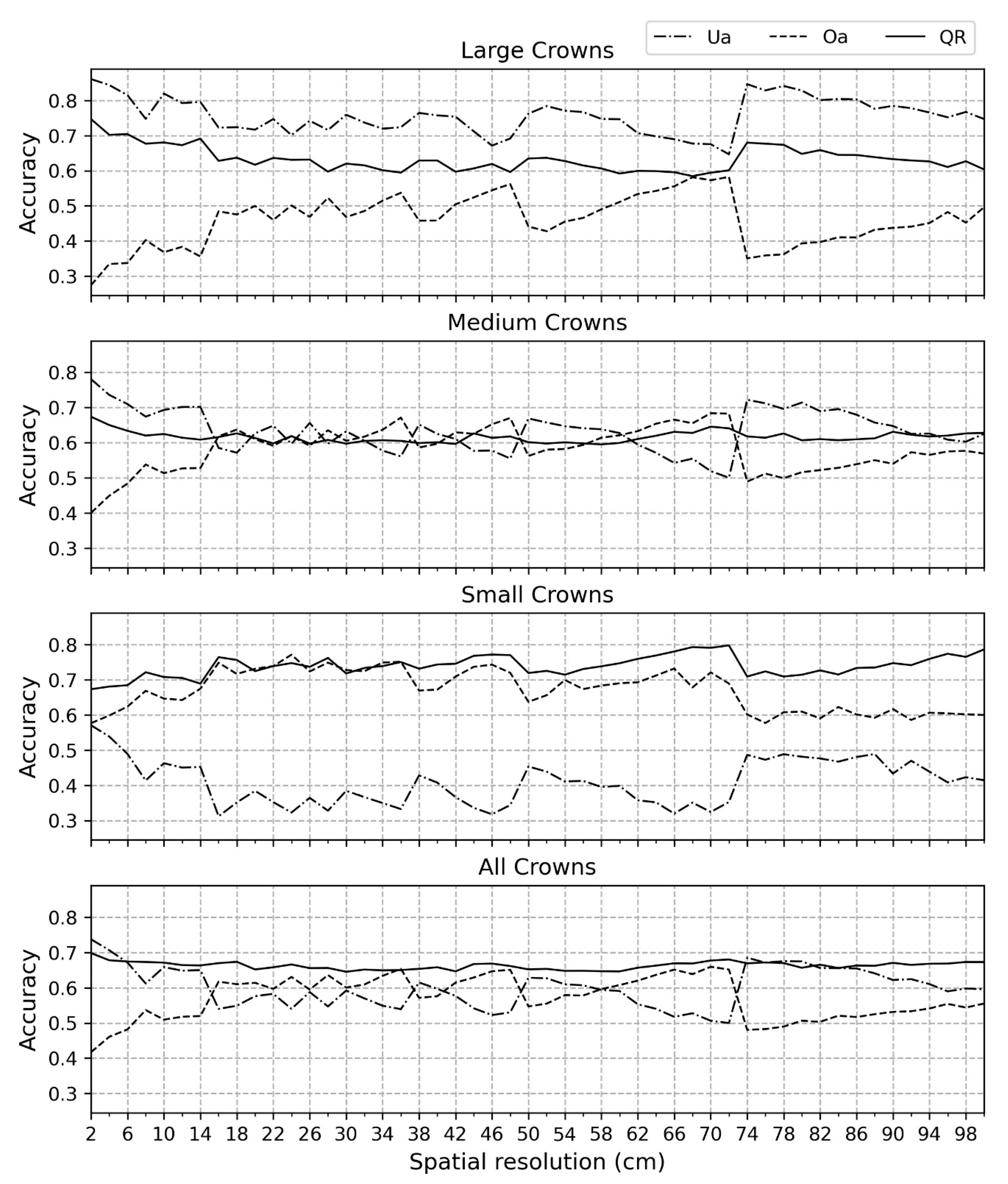
Figure 4 demonstrates the results from study site #2 using the lightness band as the segmenting data. A similar trend is shown as in Figure 2. The minor difference is that the values of Oa are lower with higher Ua, resulting in a broader gap in the large group. The best spatial resolution for segmentation is 68, 58, 2, and 30 cm for the large, medium, small, and all groups, respectively.
The results in Figure 5 resemble those in Figure 3, and the differences between Figure 5 and Figure 4 are similar to those between Figure 3 and Figure 2. The best spatial resolution for segmentation is 100, 74, 74, and 74 cm for the large, medium, small, and all groups, respectively.
Table 1 further shows the average accuracy measures for all spatial resolutions. Regardless of the study sites and groups, the mean QR value is lower with a higher Ua using the lightness band as a data source compared to using CHM, although mean Oa in the small group is slightly lower. When using the lightness band, the Oa is higher with lower Ua and QR if comparing study site #1 to study #2. However, there is little difference between them in each group using CHM.
4. Discussion
This research examined and compared the accuracy of segmenting individual tree crowns from CHMs and spectral lightness bands using maker-controlled watershed segmentation. Additionally, the effects of spatial resolution, crown size, and forest type on delineation accuracy were also investigated. The Ua, Oa, and QR are widely accepted for validating segmentation and were reported as accuracy measures in this study.
This research demonstrates that single tree crowns segmented from the lightness band are more accurate than those segmented from the CHM if both data were derived from digital photogrammetry (Figure 2, Figure 3, Figure 4 and Figure 5 and Table 1)). The underlying reason is the low quality of the CHM impacted by, for example, data source or geoprocessing [30]. First, the point cloud produced through the SfM algorithm has limited ability to detect the small gaps and peaks in the crown, which gives rise to an underestimation of the upper layers of the canopy but an overestimation of the lower layers [58,59]. Second, the edges of crowns are usually darker, lower, and often obscured by surrounding trees and are, therefore, less visible in the imagery compared to higher parts of the crowns, including the treetops [32]. The SfM–MVS process relies on the computer being able to “see” features in the imagery in order to generate a 3D position (point) [60]. Fewer points would be created at the edges, which results in a relatively smoothed and underestimated DSM based on interpolation. Both these factors would lead to an undersegmented result, which is confirmed by the fact that differences between lightness band–Ua and CHM–Ua are higher than the ones between lightness band–Oa and CHM–Oa in each study site. Third, due to the characteristics of dense forest in both study sites, digital photogrammetry can only produce the point cloud from the canopy surface visible to the camera [61]. An external DTM is needed to calculate the CHM; however, the inconsistency of the spatial resolution becomes a factor [39]. Previous research focused on comparing the CHM from the LiDAR to the one derived from digital photogrammetry based on SfM [58]. This research complements the comparison between lightness and CHM, with both from digital photogrammetry. We prove that watershed segmentation using a CHM is less accurate for a dense forest than using the natural color images and suggest that a systematic error budget analysis of CHMs derived from photogrammetry based on SfM is necessary.
Results show that spatial resolution alters the accuracy of segmentation. It is worth noting that the spectral properties of the downscaled images will not be the same as an image captured with a native spatial resolution matching that of the downscaled image (i.e., an image downscaled from 2 to 30 cm is not the same as an image captured at 30 cm to begin with). However, small UAS in the United States are not legally allowed to fly higher than 122 m (legally 400 feet) above the ground and thus the maximum pixel size that can be achieved is restricted by flying height and the sensor’s properties. The best spatial resolution both for study site #1 and #2 using lightness is located at 30 cm. Comparable accuracies lie between 30 and 62 cm, and between 26 and 42 cm, respectively. The best spatial resolution for segmentation using CHM for study site #1 and #2 is 76 and 74 cm, respectively; however, the variation of accuracies due to spatial resolution is more stable. These results provide a basis for how to adopt the best spatial resolution or kernel size for smoothing filters in the future. This research also confirms that as the spatial resolution decreases, the segmentation of the large, medium, and small crowns reaches its best accuracy at various scales, which provides the implications for segmenting trees of particular interest (e.g., large trees). However, this conclusion is limited by defining the size of trees, which is usually determined by the diameter at breast height (DBH). Although the allometric function to estimate DBH from canopy width was explored in Japan by Iizuka, Yonehara, Itoh, and Kosugi [39], such a local equation does not exist for the study area.
Based on the average QR, the segmentation accuracy does not differ much between study site #1 and #2, although study site #1 has higher Oa but lower Ua. Unlike the coniferous trees, which typically follow a distinct mountainous shape, the canopies of deciduous trees are usually much flatter [12]. Multiple treetops are prone to be detected within the deciduous crown, resulting in an oversegmentation problem, which is very obvious in the large and medium crowns using lightness as the data source (Figure 4 and Figure 5, and Table 1). The minor difference in QR between study site #1 and #2 implies that the density of the forest exerts more influence on the segmentation accuracy rather than the forest type. Besides, the reconstruction of the point cloud is limited by the smoothing in the dense matching process, creating abrupt and discontinuous vertical changes in the CHM, especially for the coniferous trees in the mixed forest [30,58]. Although research on detection and segmentation of deciduous trees has increased [62,63,64], segmenting deciduous trees in high density stands based on UAS imagery is still under development.
This research also implies that the size of the sampling reference objects impacts segmentation accuracy assessment (Figure 2 and Figure 4). Previous research favored the stratified random sampling for traditional thematic classification [53,65], but the sampling design for segmentation accuracy remains unresolved [66] and which attributes (e.g., size or shape) are best for stratified sampling needs further study.
5. Conclusions
This research compared the use of a CHM with the lightness band for the delineation of individual tree crowns based on the maker-controlled watershed algorithm. It also examined how segmentation accuracy varies due to spatial resolution, crown size, and forest type. The study highlights the following conclusions. The single tree crowns segmented from the lightness band based on the marker-control watershed algorithm are more accurate than those using the CHM if both data are derived from digital photogrammetry. The best spatial resolution using lightness is 30 cm, with comparable scales between 26 and 62 cm. The best spatial resolution for segmentation using a CHM is around 75 cm. The large trees are prone to be oversegmented, while the small trees are prone to be undersegmented. The best spatial resolution for segmenting trees of different size varies. Mixed forest type dominated by either deciduous or coniferous does not show much difference in accuracy. Finally, this research suggests that the size of the reference polygons impacts segmentation accuracy assessment, which deserves more investigation in the future.
Author Contributions
J.G., H.G., and R.G.C. conceived and designed the experiments. J.G. performed the experiments and analyzed the data with guidance from R.G.C.; J.G. wrote the paper. H.G. and R.G.C. edited and finalized the paper and manuscript. All authors have read and agreed to the published version of the manuscript.
Funding
Partial funding was provided by the New Hampshire Agricultural Experiment Station. This is Scientific Contribution Number: #2856. This work was supported by the USDA National Institute of Food and Agriculture McIntire Stennis Project #NH00095-M (Accession #1015520).
Acknowledgments
The authors would like to acknowledge Vincent Pagano, Hannah Stewart, and Benjamin Fraser for their assistance with the reference data collection.
Conflicts of Interest
The authors declare no conflict of interest.
References
- Devi, R.M.; Patasaraiya, M.K.; Sinha, B.; Saran, S.; Dimri, A.P.; Jaiswal, R. Understanding the linkages between climate change and forest. Curr. Sci. 2018, 114, 987–996. [Google Scholar] [CrossRef]
- Mitchard, E.T.A. The tropical forest carbon cycle and climate change. Nature 2018, 559, 527–534. [Google Scholar] [CrossRef] [PubMed]
- Llopart, M.; Reboita, M.S.; Coppola, E.; Giorgi, F.; da Rocha, R.P.; de Souza, D.O. Land Use Change over the Amazon Forest and Its Impact on the Local Climate. Water 2018, 10, 149. [Google Scholar] [CrossRef] [Green Version]
- Ling, P.Y.; Baiocchi, G.; Huang, C.Q. Estimating annual influx of carbon to harvested wood products linked to forest management activities using remote sensing. Clim. Chang. 2016, 134, 45–58. [Google Scholar] [CrossRef]
- Rodriguez-Gonzalez, P.M.; Albuquerque, A.; Martinez-Almarza, M.; Diaz-Delgado, R. Long-term monitoring for conservation management: Lessons from a case study integrating remote sensing and field approaches in floodplain forests. J. Environ. Manag. 2017, 202, 392–402. [Google Scholar] [CrossRef]
- Vauhkonen, J.; Imponen, J. Unsupervised classification of airborne laser scanning data to locate potential wildlife habitats for forest management planning. Forestry 2016, 89, 350–363. [Google Scholar] [CrossRef] [Green Version]
- Tomppo, E.; Malimbwi, R.; Katila, M.; Mäkisara, K.; Henttonen, H.M.; Chamuya, N.; Zahabu, E.; Otieno, J. A sampling design for a large area forest inventory: Case Tanzania. Can. J. For. Res. 2014, 44, 931–948. [Google Scholar] [CrossRef]
- Bergseng, E.; Orka, H.O.; Naesset, E.; Gobakken, T. Assessing forest inventory information obtained from different inventory approaches and remote sensing data sources. Ann. For. Sci. 2015, 72, 33–45. [Google Scholar] [CrossRef] [Green Version]
- Wagner, F.H.; Ferreira, M.P.; Sanchez, A.; Hirye, M.C.M.; Zortea, M.; Gloor, E.; Phillips, O.L.; de Souza Filho, C.R.; Shimabukuro, Y.E.; Aragao, L.E.O.C. Individual tree crown delineation in a highly diverse tropical forest using very high resolution satellite images. ISPRS J. Photogramm. Remote Sens. 2018, 145, 362–377. [Google Scholar] [CrossRef]
- Chen, G.; Weng, Q.; Hay, G.J.; He, Y. Geographic object-based image analysis (GEOBIA): Emerging trends and future opportunities. GISci. Remote Sens. 2018, 55, 159–182. [Google Scholar] [CrossRef]
- Wang, Y.; Lehtomäki, M.; Liang, X.; Pyörälä, J.; Kukko, A.; Jaakkola, A.; Liu, J.; Feng, Z.; Chen, R.; Hyyppä, J. Is field-measured tree height as reliable as believed—A comparison study of tree height estimates from field measurement, airborne laser scanning and terrestrial laser scanning in a boreal forest. ISPRS J. Photogramm. Remote Sens. 2019, 147, 132–145. [Google Scholar] [CrossRef]
- Ke, Y.; Quackenbush, L.J. A review of methods for automatic individual tree-crown detection and delineation from passive remote sensing. Int. J. Remote Sens. 2011, 32, 4725–4747. [Google Scholar] [CrossRef]
- Sačkov, I.; Santopuoli, G.; Bucha, T.; Lasserre, B.; Marchetti, M. Forest Inventory Attribute Prediction Using Lightweight Aerial Scanner Data in a Selected Type of Multilayered Deciduous Forest. Forests 2016, 7, 307. [Google Scholar] [CrossRef] [Green Version]
- Ke, Y.; Quackenbush, L.J.; Im, J. Synergistic use of QuickBird multispectral imagery and LIDAR data for object-based forest species classification. Remote Sens. Environ. 2010, 114, 1141–1154. [Google Scholar] [CrossRef]
- Pu, R.; Landry, S. A comparative analysis of high spatial resolution IKONOS and WorldView-2 imagery for mapping urban tree species. Remote Sens. Environ. 2012, 124, 516–533. [Google Scholar] [CrossRef]
- Hansen, M.C.; Potapov, P.V.; Goetz, S.J.; Turubanova, S.; Tyukavina, A.; Krylov, A.; Kommareddy, A.; Egorov, A. Mapping tree height distributions in Sub-Saharan Africa using Landsat 7 and 8 data. Remote Sens. Environ. 2016, 185, 221–232. [Google Scholar] [CrossRef] [Green Version]
- Ploton, P.; Barbier, N.; Couteron, P.; Antin, C.M.; Ayyappan, N.; Balachandran, N.; Barathan, N.; Bastin, J.F.; Chuyong, G.; Dauby, G.; et al. Toward a general tropical forest biomass prediction model from very high resolution optical satellite images. Remote Sens. Environ. 2017, 200, 140–153. [Google Scholar] [CrossRef]
- Yilmaz, V.; Yilmaz, C.S.; Tasci, L.; Gungor, O. Determination of Tree Crown Diameters with Segmentation of a UAS-Based Canopy Height Model. IPSI BGD Trans. Internet Res. 2017, 13, 63–67. [Google Scholar]
- Liu, G.J.; Wang, J.L.; Dong, P.L.; Chen, Y.; Liu, Z.Y. Estimating Individual Tree Height and Diameter at Breast Height (DBH) from Terrestrial Laser Scanning (TLS) Data at Plot Level. Forests 2018, 9, 398. [Google Scholar] [CrossRef] [Green Version]
- Gaetano, R.; Masi, G.; Poggi, G.; Verdoliva, L.; Scarpa, G. Marker-Controlled Watershed-Based Segmentation of Multiresolution Remote Sensing Images. IEEE Trans. Geosci. Remote Sens. 2015, 53, 2987–3004. [Google Scholar] [CrossRef]
- Chen, S.; Luo, J.C.; Shen, Z.F.; Hu, X.D.; Gao, L.J. Segmentation of Multi-spectral Satellite Images Based on Watershed Algorithm. In Proceedings of the 2008 International Symposium on Knowledge Acquisition and Modeling, Wuhan, China, 21–22 December 2008; pp. 684–688. [Google Scholar] [CrossRef]
- Huang, H.Y.; Li, X.; Chen, C.C. Individual Tree Crown Detection and Delineation from Very-High-Resolution UAV Images Based on Bias Field and Marker-Controlled Watershed Segmentation Algorithms. IEEE J. Sel. Top. Appl. Earth Obs. Remote Sens. 2018, 11, 2253–2262. [Google Scholar] [CrossRef]
- Cai, Y.Q.; Tong, X.H.; Shu, R.; IEEE. Multi-scale Segmentation of Remote Sensing Image Based on Watershed Transformation. In Proceedings of the 2009 Joint Urban Remote Sensing Event, Shanghai, China, 20–22 May 2009; p. 425. [Google Scholar] [CrossRef]
- Li, D.R.; Zhang, G.F.; Wu, Z.C.; Yi, L.N. An Edge Embedded Marker-Based Watershed Algorithm for High Spatial Resolution Remote Sensing Image Segmentation. IEEE Trans. Image Process. 2010, 19, 2781–2787. [Google Scholar] [CrossRef] [PubMed]
- Mylonas, S.; Stavrakoudis, D.; Theocharis, J.; Mastorocostas, P. A Region-Based GeneSIS Segmentation Algorithm for the Classification of Remotely Sensed Images. Remote Sens. 2015, 7, 2474–2508. [Google Scholar] [CrossRef] [Green Version]
- Wang, M.; Li, R. Segmentation of High Spatial Resolution Remote Sensing Imagery Based on Hard-Boundary Constraint and Two-Stage Merging. IEEE Trans. Geosci. Remote Sens. 2014, 52, 5712–5725. [Google Scholar] [CrossRef]
- Fang, F.; Im, J.; Lee, J.; Kim, K. An improved tree crown delineation method based on live crown ratios from airborne LiDAR data. Gisci. Remote Sens. 2016, 53, 402–419. [Google Scholar] [CrossRef]
- Mohan, M.; Silva, C.A.; Klauberg, C.; Jat, P.; Catts, G.; Cardil, A.; Hudak, A.T.; Dia, M. Individual Tree Detection from Unmanned Aerial Vehicle (UAV) Derived Canopy Height Model in an Open Canopy Mixed Conifer Forest. Forests 2017, 8, 340. [Google Scholar] [CrossRef] [Green Version]
- Wallace, L.; Lucieer, A.; Watson, C.S. Evaluating Tree Detection and Segmentation Routines on Very High Resolution UAV LiDAR Data. IEEE Trans. Geosci. Remote Sens. 2014, 52, 7619–7628. [Google Scholar] [CrossRef]
- Lisein, J.; Pierrot-Deseilligny, M.; Bonnet, S.; Lejeune, P. A Photogrammetric Workflow for the Creation of a Forest Canopy Height Model from Small Unmanned Aerial System Imagery. Forests 2013, 4, 922–944. [Google Scholar] [CrossRef] [Green Version]
- Planck, N.R.V.; Finley, A.O.; Kershaw, J.A.; Weiskittel, A.R.; Kress, M.C. Hierarchical Bayesian models for small area estimation of forest variables using LiDAR. Remote Sens. Environ. 2018, 204, 287–295. [Google Scholar] [CrossRef]
- Wallace, L.; Lucieer, A.; Malenovsky, Z.; Turner, D.; Vopenka, P. Assessment of Forest Structure Using Two UAV Techniques: A Comparison of Airborne Laser Scanning and Structure from Motion (SfM) Point Clouds. Forests 2016, 7, 62. [Google Scholar] [CrossRef] [Green Version]
- Zhang, J.; Lin, X. Advances in fusion of optical imagery and LiDAR point cloud applied to photogrammetry and remote sensing. Int. J. Image Data Fusion 2017, 8, 1–31. [Google Scholar] [CrossRef]
- Wang, M.; Dong, Z.P.; Cheng, Y.F.; Li, D.R. Optimal Segmentation of High-Resolution Remote Sensing Image by Combining Superpixels With the Minimum Spanning Tree. IEEE Trans. Geosci. Remote Sens. 2018, 56, 228–238. [Google Scholar] [CrossRef]
- Li, Z.; Hayward, R.; Zhang, J.; Liu, Y. Individual Tree Crown Delineation Techniques for Vegetation Management in Power Line Corridor. In Proceedings of the 2008 Digital Image Computing: Techniques and Applications, Canberra, ACT, Australia, 1–3 December 2008; pp. 148–154. [Google Scholar]
- Milas, A.S.; Arend, K.; Mayer, C.; Simonson, M.A.; Mackey, S. Different colours of shadows: Classification of UAV images. Int. J. Remote Sens. 2017, 38, 3084–3100. [Google Scholar] [CrossRef]
- SenseFly User-Manuals. Available online: https://www.sensefly.com/my-sensefly/user-manuals/ (accessed on 29 April 2020).
- Agisoft Metashape User Manual Professional Edition 1.6. Available online: https://www.agisoft.com/pdf/metashape-pro_1_6_en.pdf (accessed on 29 April 2020).
- Iizuka, K.; Yonehara, T.; Itoh, M.; Kosugi, Y. Estimating Tree Height and Diameter at Breast Height (DBH) from Digital Surface Models and Orthophotos Obtained with an Unmanned Aerial System for a Japanese Cypress (Chamaecyparis obtusa) Forest. Remote Sens. 2018, 10, 13. [Google Scholar] [CrossRef] [Green Version]
- Fraser, B.T.; Congalton, R.G. Issues in Unmanned Aerial Systems (UAS) Data Collection of Complex Forest Environments. Remote Sens. 2018, 10, 908. [Google Scholar] [CrossRef] [Green Version]
- Poblete-Echeverría, C.; Olmedo, G.; Ingram, B.; Bardeen, M. Detection and Segmentation of Vine Canopy in Ultra-High Spatial Resolution RGB Imagery Obtained from Unmanned Aerial Vehicle (UAV): A Case Study in a Commercial Vineyard. Remote Sens. 2017, 9, 268. [Google Scholar] [CrossRef] [Green Version]
- Chen, Y.; Hou, C.; Tang, Y.; Zhuang, J.; Lin, J.; He, Y.; Guo, Q.; Zhong, Z.; Lei, H.; Luo, S. Citrus Tree Segmentation from UAV Images Based on Monocular Machine Vision in a Natural Orchard Environment. Sensors 2019, 19, 5558. [Google Scholar] [CrossRef] [PubMed] [Green Version]
- GRANIT LiDAR Distribution Site. Available online: http://lidar.unh.edu/map/ (accessed on 29 April 2020).
- ESRI ArcGIS Pro 2.4.2. Available online: https://www.esri.com/en-us/arcgis/products/arcgis-pro/resources (accessed on 21 May 2020).
- Belgiu, M.; Dragut, L. Comparing supervised and unsupervised multiresolution segmentation approaches for extracting buildings from very high resolution imagery. ISPRS J. Photogramm. Remote Sens. 2014, 96, 67–75. [Google Scholar] [CrossRef] [PubMed] [Green Version]
- Wulder, M.; Niemann, K.O.; Goodenough, D.G. Local Maximum Filtering for the Extraction of Tree Locations and Basal Area from High Spatial Resolution Imagery. Remote Sens. Environ. 2000, 73, 103–114. [Google Scholar] [CrossRef]
- Zhang, Y.; Feng, X.; Le, X. Segmentation on Multispectral Remote Sensing Image Using Watershed Transformation. In Proceedings of the 2008 Congress on Image and Signal Processing, Hainan, China, 27–30 May 2008; pp. 773–777. [Google Scholar]
- Kornilov, S.A.; Safonov, V.I. An Overview of Watershed Algorithm Implementations in Open Source Libraries. J. Imaging 2018, 4, 123. [Google Scholar] [CrossRef] [Green Version]
- Polewski, P.; Yao, W.; Cao, L.; Gao, S. Marker-free coregistration of UAV and backpack LiDAR point clouds in forested areas. ISPRS J. Photogramm. Remote Sens. 2019, 147, 307–318. [Google Scholar] [CrossRef]
- Xiao, P.F.; Feng, X.Z.; Zhao, S.H.; Me, S.J.; Wang, P.F.; Badawi, R. Applying texture marker-controlled watershed transform to the segmentation of IKONOS image. In Geoinformatics 2007: Remotely Sensed Data and Information, Pts 1 and 2; Ju, W., Zhao, S., Eds.; SPIE: Bellingham, WA, USA, 2007; Volume 6752. [Google Scholar]
- Furnari, A.; Farinella, G.M.; Bruna, A.R.; Battiato, S. Distortion adaptive Sobel filters for the gradient estimation of wide angle images. J. Vis. Commun. Image Represent. 2017, 46, 165–175. [Google Scholar] [CrossRef]
- van der Walt, S.; Schönberger, J.L.; Nunez-Iglesias, J.; Boulogne, F.; Warner, J.D.; Yager, N.; Gouillart, E.; Yu, T. scikit-image: Image processing in Python. PeerJ 2014, 2, e453. [Google Scholar] [CrossRef] [PubMed]
- Congalton, R.G.; Green, K. Assessing the Accuracy of Remotely Sensed Data: Principles and Practices, 3rd ed.; CRC Press: Boca Raton, FL, USA, 2019. [Google Scholar]
- Yang, J.; He, Y.; Caspersen, J. Region merging using local spectral angle thresholds: A more accurate method for hybrid segmentation of remote sensing images. Remote Sens. Environ. 2017, 190, 137–148. [Google Scholar] [CrossRef]
- Möller, M.; Lymburner, L.; Volk, M. The comparison index: A tool for assessing the accuracy of image segmentation. Int. J. Appl. Earth Obs. Geoinf. 2007, 9, 311–321. [Google Scholar] [CrossRef]
- Chen, Y.Y.; Ming, D.P.; Zhao, L.; Lv, B.R.; Zhou, K.Q.; Qing, Y.Z. Review on High Spatial Resolution Remote Sensing Image Segmentation Evaluation. Photogramm. Eng. Remote Sens. 2018, 84, 629–646. [Google Scholar] [CrossRef]
- Weidner, U. Contribution to the assessment of segmentation quality for remote sensing applications. Int. Arch. Photogramm. Remote Sens. 2008, 37, 479–484. [Google Scholar]
- Jayathunga, S.; Owari, T.; Tsuyuki, S. Evaluating the Performance of Photogrammetric Products Using Fixed-Wing UAV Imagery over a Mixed Conifer–Broadleaf Forest: Comparison with Airborne Laser Scanning. Remote Sens. 2018, 10, 187. [Google Scholar] [CrossRef] [Green Version]
- Vastaranta, M.; Wulder, M.; White, J.; Pekkarinen, A.; Tuominen, S.; Ginzler, C.; Kankare, V.; Holopainen, M.; Hyyppä, J.; Hyyppä, H. Airborne laser scanning and digital stereo imagery measures of forest structure: Comparative results and implications to forest mapping and inventory update. Can. J. Remote Sens. 2013, 39, 382–395. [Google Scholar] [CrossRef]
- Iglhaut, J.; Cabo, C.; Puliti, S.; Piermattei, L.; O’Connor, J.; Rosette, J. Structure from Motion Photogrammetry in Forestry: A Review. Curr. For. Rep. 2019, 5, 155–168. [Google Scholar] [CrossRef] [Green Version]
- Matese, A.; Di Gennaro, S.F.; Berton, A. Assessment of a canopy height model (CHM) in a vineyard using UAV-based multispectral imaging. Int. J. Remote Sens. 2017, 38, 2150–2160. [Google Scholar] [CrossRef]
- Nuijten, J.G.R.; Coops, C.N.; Goodbody, R.H.T.; Pelletier, G. Examining the Multi-Seasonal Consistency of Individual Tree Segmentation on Deciduous Stands Using Digital Aerial Photogrammetry (DAP) and Unmanned Aerial Systems (UAS). Remote Sens. 2019, 11, 739. [Google Scholar] [CrossRef] [Green Version]
- Ene, L.; Næsset, E.; Gobakken, T. Single tree detection in heterogeneous boreal forests using airborne laser scanning and area-based stem number estimates. Int. J. Remote Sens. 2012, 33, 5171–5193. [Google Scholar] [CrossRef]
- Hamraz, H.; Contreras, M.A.; Zhang, J. A robust approach for tree segmentation in deciduous forests using small-footprint airborne LiDAR data. Int. J. Appl. Earth Obs. Geoinf. 2016, 52, 532–541. [Google Scholar] [CrossRef] [Green Version]
- Stehman, S.V. Sampling designs for accuracy assessment of land cover. Int. J. Remote Sens. 2009, 30, 5243–5272. [Google Scholar] [CrossRef]
- Ye, S.; Pontius, R.G.; Rakshit, R. A review of accuracy assessment for object-based image analysis: From per-pixel to per-polygon approaches. ISPRS J. Photogramm. Remote Sens. 2018, 141, 137–147. [Google Scholar] [CrossRef]
Figure 1.
Study sites at College Woods, New Hampshire, USA

Figure 2.
Impact of spatial resolution and crown size on Oa, Ua, and QR using the lightness band in study site #1.
Figure 2.
Impact of spatial resolution and crown size on Oa, Ua, and QR using the lightness band in study site #1.

Figure 3.
Impact of spatial resolution and crown size on Oa, Ua, and QR using the canopy height model (CHM) in study site #1.
Figure 3.
Impact of spatial resolution and crown size on Oa, Ua, and QR using the canopy height model (CHM) in study site #1.

Figure 4.
Impact of spatial resolution and crown size on Oa, Ua, and QR using the lightness band in study site #2.
Figure 4.
Impact of spatial resolution and crown size on Oa, Ua, and QR using the lightness band in study site #2.

Figure 5.
Impact of spatial resolution and crown size on Oa, Ua, and QR using the CHM in study site #2.
Figure 5.
Impact of spatial resolution and crown size on Oa, Ua, and QR using the CHM in study site #2.


Table 1.
Average accuracy measures of all spatial resolutions using lightness or CHM from each study site.
Table 1.
Average accuracy measures of all spatial resolutions using lightness or CHM from each study site.
| Group | Study Site #1 | Study Site #2 | ||||||||||
|---|---|---|---|---|---|---|---|---|---|---|---|---|
| Lightness | CHM | Lightness | CHM | |||||||||
| Oa | Ua | QR | Oa | Ua | QR | Oa | Ua | QR | Oa | Ua | QR | |
| Large | 0.51 | 0.73 | 0.61 | 0.48 | 0.62 | 0.70 | 0.46 | 0.76 | 0.63 | 0.47 | 0.62 | 0.70 |
| Medium | 0.63 | 0.59 | 0.62 | 0.58 | 0.41 | 0.76 | 0.58 | 0.63 | 0.62 | 0.56 | 0.46 | 0.75 |
| Small | 0.70 | 0.40 | 0.73 | 0.71 | 0.22 | 0.86 | 0.67 | 0.41 | 0.74 | 0.70 | 0.21 | 0.87 |
| All | 0.62 | 0.57 | 0.65 | 0.59 | 0.42 | 0.78 | 0.57 | 0.60 | 0.66 | 0.57 | 0.43 | 0.77 |
© 2020 by the authors. Licensee MDPI, Basel, Switzerland. This article is an open access article distributed under the terms and conditions of the Creative Commons Attribution (CC BY) license (http://creativecommons.org/licenses/by/4.0/).
Share and Cite
MDPI and ACS Style
Gu, J.; Grybas, H.; Congalton, R.G. A Comparison of Forest Tree Crown Delineation from Unmanned Aerial Imagery Using Canopy Height Models vs. Spectral Lightness. Forests 2020, 11, 605. https://doi.org/10.3390/f11060605
AMA Style
Gu J, Grybas H, Congalton RG. A Comparison of Forest Tree Crown Delineation from Unmanned Aerial Imagery Using Canopy Height Models vs. Spectral Lightness. Forests. 2020; 11(6):605. https://doi.org/10.3390/f11060605
Chicago/Turabian StyleGu, Jianyu, Heather Grybas, and Russell G. Congalton. 2020. "A Comparison of Forest Tree Crown Delineation from Unmanned Aerial Imagery Using Canopy Height Models vs. Spectral Lightness" Forests 11, no. 6: 605. https://doi.org/10.3390/f11060605
Note that from the first issue of 2016, this journal uses article numbers instead of page numbers. See further details here.