
An Unsupervised Canopy-to-Root Pathing (UCRP) Tree Segmentation Algorithm for Automatic Forest Mapping

1
Lyles School of Civil Engineering, Purdue University, 550 Stadium Mall Drive, West Lafayette, IN 47907, USA
2
Institute for Plant Sciences, Purdue University, 915 W. State Street, West Lafayette, IN 47907, USA
3
Forestry and Natural Resources, Purdue University, 715 W. State Street, West Lafayette, IN 47907, USA
4
Environmental and Ecological Engineering, Purdue University, 500 Central Dr, West Lafayette, IN 47907, USA
*
Author to whom correspondence should be addressed.
Remote Sens. 2022, 14(17), 4274; https://doi.org/10.3390/rs14174274
Submission received: 1 August 2022
/
Revised: 25 August 2022
/
Accepted: 27 August 2022
/
Published: 30 August 2022
(This article belongs to the Special Issue Application of Remote Sensing in Agroforestry II)
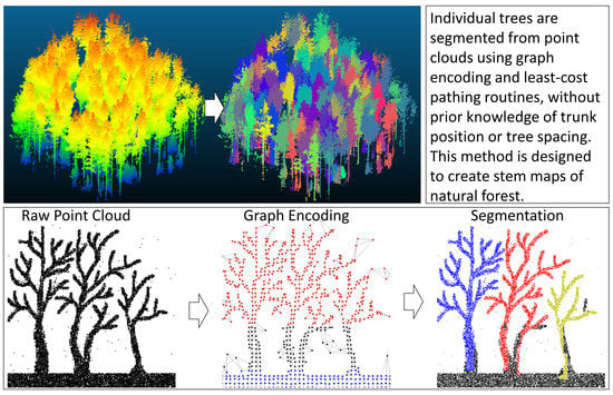
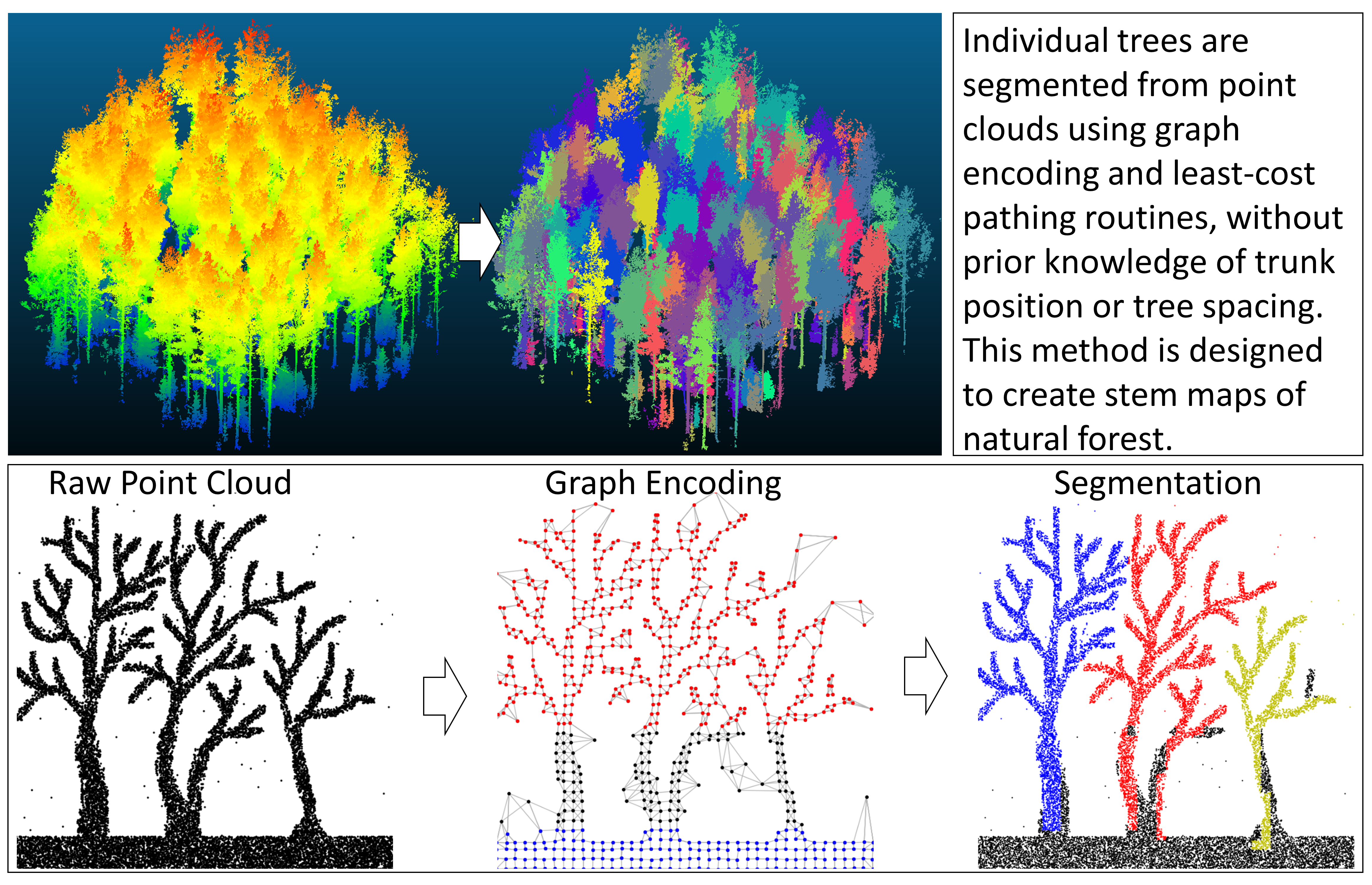
Abstract
:Terrestrial laser scanners, unmanned aerial LiDAR, and unmanned aerial photogrammetry are increasingly becoming the go-to methods for forest analysis and mapping. The three-dimensionality of the point clouds generated by these technologies is ideal for capturing the structural features of trees such as trunk diameter, canopy volume, and biomass. A prerequisite for extracting these features from point clouds is tree segmentation. This paper introduces an unsupervised method for segmenting individual trees from point clouds. Our novel, canopy-to-root, least-cost routing method segments trees in a single routine, accomplishing stem location and tree segmentation simultaneously without needing prior knowledge of tree stem locations. Testing on benchmark terrestrial-laser-scanned datasets shows that we achieve state-of-the-art performances in individual tree segmentation and stem-mapping accuracy on boreal and temperate hardwood forests regardless of forest complexity. To support mapping at scale, we test on unmanned aerial photogrammetric and LiDAR point clouds and achieve similar results. The proposed algorithm’s independence from a specific data modality, along with its robust performance in simple and complex forest environments and accurate segmentation results, make it a promising step towards achieving reliable stem-mapping capabilities and, ultimately, towards building automatic forest inventory procedures.
1. Introduction
Forest inventories provide critical data for understanding the structure, distribution, and temporal changes of trees within a forest or plantation. Inventories collect geometric and statistical characteristics of individual trees, such as tree height, diameter at breast height (DBH), canopy volume, biomass estimation, and branching structure of the tree [1,2]. These descriptors are vital for quantifying and monitoring forest health, above-ground biomass [3], vegetation density, and carbon absorption [4]. Inventory data are also necessary for business. Lumber companies remain competitive by anticipating customer demands years in advance. Making these predictions requires inventories of the number and size of trees available for immediate harvest and the growth progress of younger stands [5]. Despite the need for accurate, forest-wide inventories, the current inventory practice relies on manual measurements of a small subset of the forest and assumes features of the sample are representative of the entire forest population. The high cost of collecting these manual measurements limits the area covered by traditional forest inventories.
1.1. Image-Based Stem Mapping
For several decades, aerial imagery has been the foundation for attempts to automatically perform forest inventories [6,7,8,9]. Image-based stem mapping methods generally maximize any spectral difference between the canopy nearest the trunk and the canopy further from the trunk. These algorithms can be roughly grouped into three methods: local maxima search, valley following, and region growing.
Local maxima search locates stems by labeling clusters of local maximum points as trunk locations. In 1991, Pinz [8] introduced a method in which a moving window was passed over single-band imagery, and the local brightest pixels were marked. The assumption behind this method is that tree canopies are generally conical or spherically shaped and will thus catch more sunlight at the peak of the tree than near the edges or base. When seen from above, trees will appear as circles with bright centers. Subsequent work in this category researched the utility of alternating the size of the moving window [6].
Valley following is another approach for finding the position of individual trees. This method uses an analogous assumption to the local maxima method. Instead of finding local brightest peaks, the valley-following method attempts to trace the shaded valleys between peaks of coniferous trees [9].
With the improvement of image segmentation algorithms, region-growing algorithms, such as watershed segmentation, were applied to tree detection. Culvenor [10] used the local maxima point as a seed point and then applied region growing to segment the shaded edges of the canopy. Wang et al. [11] applied watershed segmentation to images to refine tree crowns, limiting the extent of the watershed region by the geodesic distance from the estimated trunk location.
These image-based methods suffer from several limitations. The nature of image data limits these methods to detecting basic tree parameters, such as stem location and crown delineation, of only trees tall enough to breach the upper canopy. Additionally, because the fundamental premise of these methods is that bright spots represent canopy peaks, tree spacing must be ideal. If trees are spaced too closely, no distinction can be made between individuals. If trees are spaced too far apart, grassy areas between trees can have crown-like brightness values and cause false positives [12]. Further, the quality of the stem mapping results depends on the resolution of the input data. Different post-processing or segmentation approaches are required depending on the image resolution [13].
1.2. Airborne LiDAR-Based Stem Mapping
As airborne LiDAR and other airborne ranging technologies were commercialized, the image methods discussed above began to be applied to Digital Surface Models (DSMs). Segmentation on DSMs provides better results since the values in the image represent the elevation of the top of the canopy and are no longer dependent on reflected sunlight. Lamar et al. [14] utilized watershed algorithms to map canopy extent, and Zhao et al. [7] utilized the local maxima method by applying circular moving window filters of various sizes.
While the DSM-based methods provide better results than the image-based approach described in Section 1.1, two critical problems plague all the raster-based methods so far discussed. First, neither imagery nor DSMs detect any features below the canopy—features necessary to measure when performing forest inventories. Second, both raster-based methods assume that the center of the tree will correspond to a local maximum point in the canopy. This assumption about the shape of the canopy is often valid for coniferous trees, leading most methods discussed above to be solely tested on coniferous forests where the conical shape and wide spacing of the variety make segmentation easier. However, studies that perform stem mapping over deciduous forests find a significant reduction in accuracy since deciduous canopies have minor height differences between the center and edges and tend to intertwine with neighboring trees [13].
1.3. High-Resolution Point Cloud Stem Mapping
High resolution point clouds can be generated from various technologies. Three will be discussed here: airborne LiDAR, airborne photogrammetry, and terrestrial laser scanners.
With the proliferation of laser ranging technology in the form of terrestrial laser scanners and airborne manned and unmanned systems, LiDAR has become the default choice for forest inventory automation research [15,16]. The advantage of LiDAR over aerial imagery is its ability to capture features in three dimensions, giving users the potential to measure the full range of tree features necessary to replicate forest inventories, a feat unattainable from imagery alone [17].
While airborne LiDAR is an excellent tool for capturing the structure of forests, photogrammetry is an alternative technology for creating point clouds that has some advantages over LiDAR. High-end LiDAR units can be prohibitively expensive, and less costly LiDAR units produce point clouds with significantly lower point density and higher noise levels than point clouds derived from photogrammetric techniques [18]. Both ground-based and UAV-mounted photogrammetric systems have been shown to capture tree structures with a level of detail equal to or rivaling that of laser scanning systems both in accuracy and mobility [19,20], offering a cost-effective way to create high-density, high-precision point clouds of forests. The most significant drawback to photogrammetry-based methods is their inability to penetrate the forest canopy to measure the ground surface or stem structure [21]. For this reason, photogrammetry has limited applications in stem mapping where canopies are perennial. However, in deciduous forests, the leaf-off period provides an opportunity to capture dense point clouds of the stem structure using UAV photogrammetry [22,23].
Though terrestrial laser scanners (TLS) cannot cover large areas quickly, a significant advantage of the technology over its airborne cousin is the level of detail that can be captured. TLS forest point clouds have the potential to capture detail as minute as the texture of tree bark. However, a prerequisite to extracting tree features from point clouds is segmenting the point cloud data into individual trees [2]. Segmentation is a challenging task. The complex geometry of trees, the diversity of tree structure, and the entangled nature of the forest environment, especially in natural forests, make it difficult to procedurally segment individual trees from point clouds [24].
Many methods have been proposed to segment individual trees from high-resolution point clouds [24]. These methods will be introduced in the following categories: deep learning, point density, building block, and graph-based methods. The method proposed in this paper is graph-based, so this category will be discussed in further detail. However, deep learning, point density, and building block methods will also be presented for reference.
Detecting objects in point clouds using deep learning methods is a growing area of research [25,26]. Though most research has been aimed at recognizing manmade objects, these methods have also been used for tree stem mapping and point cloud segmentation [27,28]. This approach has yielded promising results on small point cloud datasets of relatively uniform trees; however, the lack of large amounts of labeled data has been cited as a major limitation to expanding this approach [29]. An additional barrier to implementing these methods on larger data sets is the computational power needed to train and implement the models. Current methods are limited in the area that can be processed [30].
Point density methods attempt to segment individual trees by first finding tree trunks based on the hypothesis that areas of high point density and elevation correspond to trunk locations [31] and then segmenting the remaining points in the point cloud based on their relationship to the found trunk locations. A common procedure is to create a grid of two-dimensional cells in the cartesian plane (i.e., X, Y coordinates) and populate each cell with the sum of all point elevations falling within it [32]. Local maxima points are then extracted from the resulting raster. These peaks are labeled as tree trunk locations. The remaining points can then be attached to each trunk location through various methods. The most common method is to simply label each point within a given radius to the nearest trunk [32]. This point density method works well where trees are of similar size and planted in equally spaced rows as found on plantations. Here, known tree spacing can be added as prior information to improve row and tree detection [33]. This method yields poor results where trees of mixed height and size exist in the same scene. Smaller trees often have fewer points on their trunks than larger trees, making results highly dependent on the values chosen for the grid size and the thresholds used for peak detection [34].
Building block methods also follow a two-step process for tree extraction. First, probable trunks are detected as single points or clusters of points, and then a second step attempts to “grow” a tree from each trunk by iteratively selecting adjacent chunks of the point cloud and adding these chunks to the growing tree based on some criteria. Early forms of the building block method were developed for converting single-tree point clouds into a representative set of geometric shapes. Raumonen et al. [1] divided single-tree point clouds into small chunks and then, after picking a starting chunk, used these chunks to build cylindrical and linear branching features iteratively. Several methods for detecting the starting point or trunk exist, such as detecting vertical cylinders in the understory [2,35], finding vertical features by identifying clusters of points present in multiple elevation layers of the point cloud [22], and identifying clusters of points in the understory after a vegetation-filtering routine [36,37]. After detecting the starting point, or starting trunk, for each tree, the remaining points are added, usually iteratively, to the appropriate starting trunk. One method is to cluster the remaining points through voxelization and then use connected component analysis to grow each tree from the starting point [35,37]. Points can also be segmented directly by iteratively attaching each point to the trunk belonging to the nearest previously attached point [22]. With this method, better segmentation accuracy can be obtained by density-based spatial clustering where trees overlap [2].
Graph-based methods for segmenting the branching structure of trees from 3D point clouds assume that any given part of a tree must be connected by some path through the structure of the tree to the trunk and root system. Some of the first uses of graphs for modeling trees from remotely sensed data were introduced to create more realistic trees for virtual worlds [38,39]. Graphs were further adopted by Vicari et al. as a method for applying wood/leaf classification to single-tree point clouds. First, the point cloud of a tree is converted into a network of nodes and edges. Then, under the assumption that a tree is a structure that connects each leaf to the root through woody branches, the least-cost path from each node down to the root of the tree is calculated, allowing each node to be ranked based on the number of paths passing through it. High-use nodes are labeled as branches, while nodes used by few paths are labeled as vegetation [4].
Classifying woody and leafy structures from the point cloud has continued to be the major impetus for further development of graph-based classification algorithms; however, using graphs to segment individual trees has received some secondary attention. These approaches tend to work from the ground upward, starting with trunk locations found through initial processing and then growing the tree in a root-to-canopy direction using least-cost pathing. Wang [15] proposed a two-step, graph-based tree segmentation algorithm that utilized the results of wood/leaf classification to identify individual trunks within a forest point cloud and then segment trees by connecting branches and leafy structures to the nearest trunk by graph distance. In like manner, the work of Westling et al. introduced a graph-based method for isolating individual trees from multi-tree scans of orchards. This method is also a two-step process. It begins with a trunk-finding procedure followed by a least-cost pathing routine to segment trees [16]. In pursuit of automating forest inventories using point cloud data, this paper presents an unsupervised method for segmenting individual trees from point clouds. Our method introduces a novel, one-step procedure which uses least-cost routing from tree canopy points down to the ground to simultaneously segment individual trees and find trunk locations. This canopy-to-root routing direction removes the need to perform a separate trunk-detection routine. Since point clouds can be derived from multiple procedures which each present unique omissions in the data, the performance of this algorithm will be assessed on benchmark datasets collected with terrestrial laser scanners (TLS), photogrammetrically derived point clouds, and LiDAR datasets collected from unmanned aerial vehicle (UAV) platforms.
The main contributions of this study are: (1) proposing an unsupervised tree segmentation algorithm that utilizes canopy-to-root, least-cost routing to locate stem positions and segment individual trees; (2) exceeding the accuracy of the state-of-the-art unsupervised forest segmentation methods; (3) yielding a minimal decrease in segmentation accuracy on high-complexity forest areas; (4) testing the proposed algorithm on point clouds derived from three sensor types—UAV-based photogrammetry, terrestrial laser scanning, and aerial LiDAR—showing that the proposed method is useful regardless of the mapping system employed; and (5) testing the proposed algorithm on point clouds of various forest types: boreal and temperate hardwood and both natural forests and plantations.
2. Materials and Methods
2.1. Datasets
Complicating the task of individual tree segmentation are the dissimilarities between point clouds derived from various methods. Terrestrial laser scanners produce highly accurate point clouds, but the spacing between points (the point density) decreases with distance from the sensor, and lower branches often occlude areas of the upper canopy [2]. Airborne LiDAR produces point clouds with less variation in point density, but the upper canopy often occludes the trunk detail [25]. An additional source of point cloud data only briefly discussed in tree segmentation literature is UAV-based photogrammetry, which produces point clouds with unique point distributions and omissions but has been shown to yield useful results [35].
This study used multiple point cloud datasets to validate the results of the tree-stem-mapping and segmentation method presented. These point cloud datasets were captured using three distinct technologies—TLS, UAV-based photogrammetry, and UAV-based LiDAR. Each dataset was accompanied by a manually created tree map which encodes the height and position of every tree in the dataset. This tree map was used to validate the results of tree stem mapping and segmentation.
2.1.1. TLS Datasets
The TLS datasets used in this study were acquired from the International TLS Benchmarking project, organized by the Finnish Geospatial Research Institute [24]. Each of the six publicly available datasets used here captures a separate 32 m × 32 m forest plot in the southern boreal forest of Evo, Finland. The dominant tree species in the plots are Scots pine, Norway spruce, silver birch, and downy birch. Researchers from the University of Helsinki, Finland, collected the data in April and May of 2014. Each plot was covered with five stationary scans using a Leica HDS6100 terrestrial laser scanner with a field of view of 360° × 310° and accuracy of ±2 mm at 25 m. These were combined into a multi-scan point cloud in post-processing using spherical targets. The final point clouds have an approximate horizontal point density of 125 K points/m2. Each dataset is accompanied by a digital terrain model (DTM) extracted from the multi-scan point cloud and a tree map that includes positions, heights, and diameters at breast height (DBH) of all trees in the plot whose DBHs are greater than 5 cm. Tree positions were manually measured by the researchers from the multi-scan point clouds at the center of the trunk at breast height; heights were measured with a hypsometer to a resolution of 10 cm; and DBHs were measured with steel calipers. Two plots are categorized as easy to segment, two as intermediate to segment, and the remaining two as difficult to segment. These categories were designated intuitively based on stem visibility at ground level, stem density, and variation of DBH [24]. For reference, Figure 1 shows a cross-section of a representative from each category of plot. This International TLS Benchmarking data set has been used by multiple researchers to test tree stem mapping algorithms [2,15,37].
A limitation of this dataset is that tree features are only provided for trees whose DBHs exceeded 5 cm. It is apparent, by visual inspection of the point cloud, that many trees exist in the scanned plots whose DBHs are less than 5 cm. Thus, to avoid the validation errors which small vegetation caused in previous work [15], steps must be taken to exclude small trees from the segmentation results so that the results match the limitations of the validation data sets. However, filtering segmentation results by DBH requires an additional procedure to be developed for automatically detecting the DBH of segmented trees. Segmentation validation results are then greatly affected by the accuracy of the secondary filtering step. Instead of introducing error by attempting to filter segmentation results, we used the point clouds to manually measure the tree positions and of the trees smaller than 5 cm and added these positions to the provided validation data. This step removed the need to filter segmentation results since the combined validation data included the position and height of every tree in the raw data which could be detected by human inspection regardless of DBH. Thus, we disregarded the provided DBH measurements and did not consider DBH in the validation of the proposed algorithm.
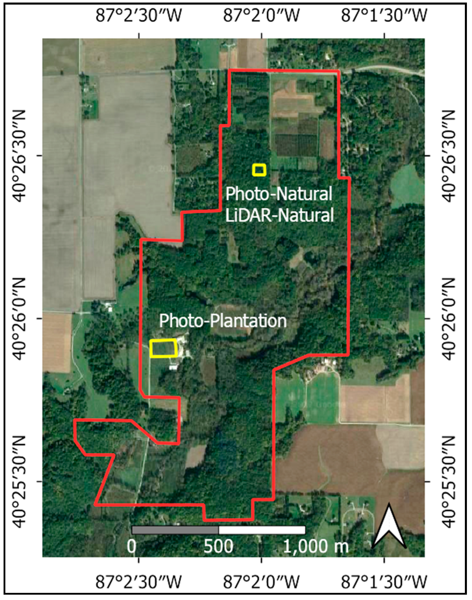
2.1.2. Martell Forest
In addition to the TLS data sets, UAV LiDAR and UAV Photogrammetric data sets were collected over portions of Martell Forest, a research forest in northern Indiana, USA (40.44105, −87.03353). Figure 2 shows the positions of each sample site within Martell Forest.
Both the Photo-Natural and LiDAR-Natural data sets were collected over the same 58 m × 58 m portion of the Martell Forest. This site is a natural forest area comprised mostly of oak and hickory species with a maximum tree height of 34 m.
The Photo-Plantation dataset was collected over a 65 m × 130 m plantation of mature walnut trees in Martell Forest. This plantation features regularly spaced trees on a mowed lawn. Trees on this site reach a maximum height of 24 m.
2.1.3. UAV LiDAR Datasets
TLS point clouds collected from stationary or mobile devices produce highly detailed models of the forest environment [16,40]. However, these methods are limited in spatial coverage. Aerial LiDAR mounted to UAV platforms can cover large, forested areas quickly. While aerial LiDAR is the preferred data collection technique for forest mapping because of its ability to penetrate the canopy, details of the stem structure are still highly limited when leaves are present [31]; thus, we collected lidar data during the leaf off-season.
To create the LiDAR-Natural dataset, we used a Matrice 300 platform mounted with a Zenmuse L1 lidar sensor (DJI, Shenzhen, China) for aerial lidar acquisition. The flight mission was conducted on 1 April 2022. The flight parameters of the UAV LiDAR mission are presented in Table 1. The Zenmuse L1 sensor is comprised of the Livox Avia LiDAR sensor and Bosch BMI088 inertial measurement unit housed and mounted on a 3-axis gimbal. The sensor is integrated with the Matrice 300′s onboard RTK system. The trajectory and final point cloud are computed using the DJI Terra software. While the accuracy of any specific point varies with altitude, the reflectivity of the surface, and scan angle, the system is rated as having a horizontal accuracy of 10 cm and a vertical accuracy of 5 cm at 50 m altitude [18]. The resulting point cloud contains 2.2 million points with an approximate horizontal point density of about 670 points/m2.
To validate segmentation results, a tree map was built of the site. The point cloud was used to manually measure the position and height of each tree visible in the data. Two details should be noted concerning this validation tree map. First, we did not attempt to make on-the-ground measurements of tree positions—only the positions of trees that a human could distinguish in the data were used for validation. Second, no size restriction was placed on what features in the data should be considered as trees; if a feature was visible in the point cloud data that a human investigator would term a ‘tree’, that feature was marked in the validation tree map and we expected our proposed algorithm to detect the feature.
2.1.4. UAV Photogrammetric Datasets
To build a photogrammetric validation dataset, we used a Matrice 300 platform mounted with a Zenmuse P1 RGB camera (DJI, Shenzhen, China) for image acquisition. Two flight missions were conducted. The first, Photo-Plantation, was flown on 3 March 2021. The second, Photo-Natural, was flown on 17 April 2021. Photo-Natural was collected over the same section of Martell Forest as LiDAR-Natural. The flight parameters of the photogrammetric flights are presented in Table 2.
We utilized the INCORS INWL base station maintained by the Indiana Department of Transportation and the Matrice’s RTK capabilities to do direct georeferencing on the images. Five ground control points (GCPs) were also deployed to check for any horizontal shift in the absolute coordinates of the data. The GCPs were surveyed with a Trimble R10 survey-grade GNSS receiver also utilizing the INCORS INWL base station for RTK positioning.
The images were processed using the photogrammetric processing software Agisoft Metashape (version 1.7.1) (Agisoft, St. Petersburg, Russia). We followed the four-step processing procedure available in Metashape: align photos, build dense point cloud, build DEM, and build orthomosaic. The ‘high accuracy’ option was used to align photos. ‘Mild depth filtering’ was implemented by Metashape while building the dense point cloud. The DEM and orthomosaic were created, and the orthomosaic was used to extract the GCP coordinates as computed in the photogrammetric reconstruction. These coordinates were then compared to the surveyed coordinates of the GCPs to calculate horizontal and vertical shift errors. The absolute shift error was found to be . The dense point cloud was then exported in the LAS format, and a correction for the shift error was applied using an in-house-developed python script. The resulting photogrammetric point cloud contains 13.4 million points with an approximate horizontal point density of 16 K points/m2.
To validate the segmentation results, a tree map was built for each photogrammetric data set. The point clouds were used to manually measure the position and height of each tree visible in the data.
2.2. Segmentation Method
The algorithm proposed in this paper is founded on the assumption that, given a graph-space encoding of a forest point cloud and a properly crafted cost function, the route of least cost from any given point in the forest canopy to the ground will pass through the trunk of the tree to which the canopy point belongs. The implementation presented consists of a series of point cloud preprocessing steps followed by the graph-building and pathfinding segmentation procedure. The process can be divided into six processing steps: (1) Point Cloud Normalization, where the terrain elevation is subtracted from each point in the point cloud to remove the effect of the terrain; (2) Superpoint Encoding, where superpoints are created by aggregating the properties of all points within voxel cells into a single superpoint; (3) Rough Classification, where the height of a superpoint above the ground is used to identify ground points and canopy points; (4) Network Construction, where the cloud of superpoints is converted into a graph space by using superpoints as nodes and defining edge connections between nodes; (5) Least-cost Routing, in which the least-cost route from each canopy superpoint down to the first ground superpoint is traced and branching network structures are built by linking all routes which end at the same ground superpoint; and finally (6) Final Segmentation, where neighboring branching structures are combined into tree-like networks and each tree-like network is assigned a label that is recursively applied to all superpoints connected by the tree-like network and then to all original points encoded by each superpoint. These steps are described in further detail in the following subsections.
2.2.1. Point Cloud Normalization
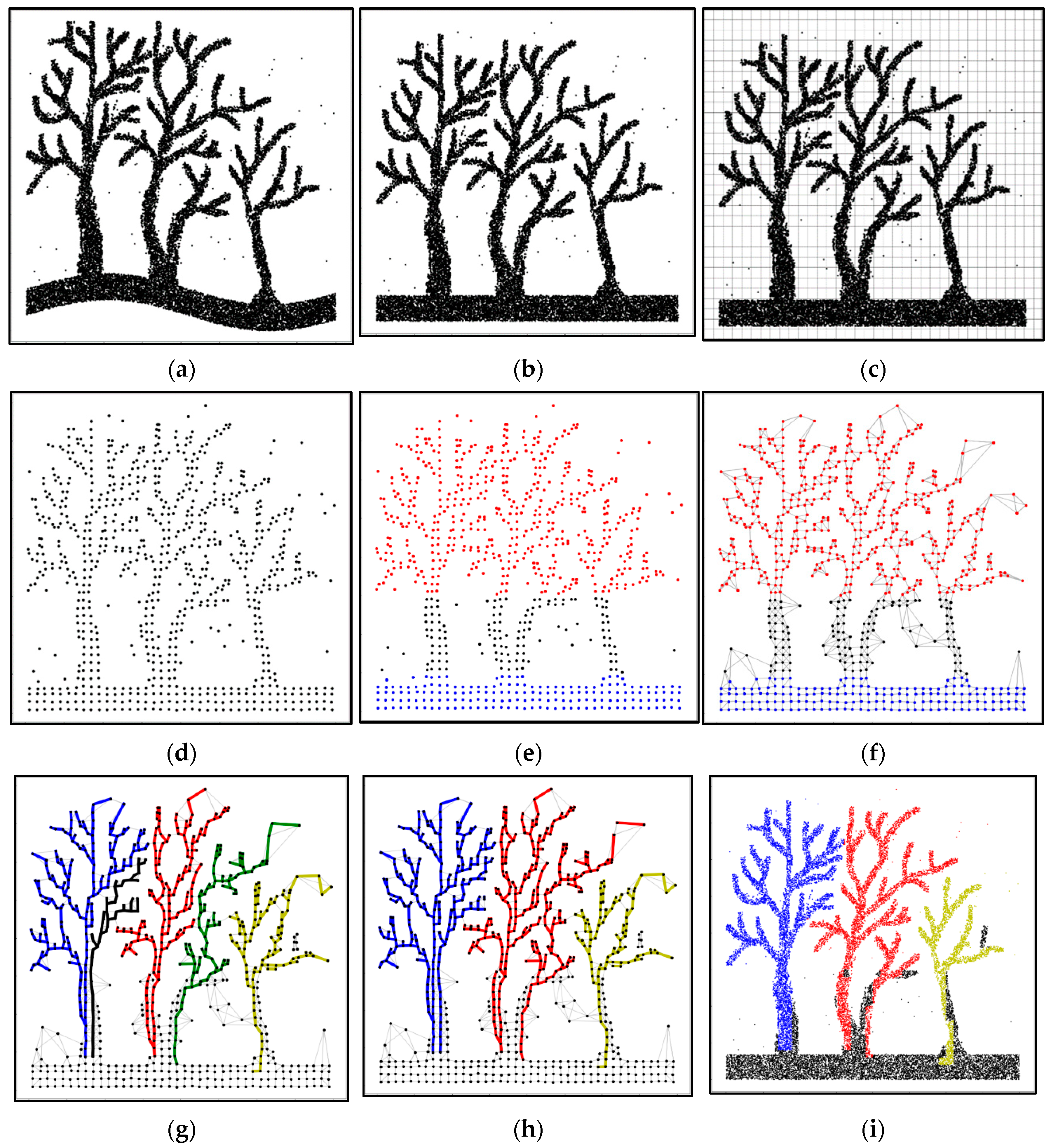
Before processing, the point cloud input data must be normalized to remove the effect of the terrain. This pre-processing step is precedented in the literature [4,16,31]. Along with the point cloud, the user of this proposed algorithm provides a DTM which encodes the elevation of the terrain in a regular grid pattern. For each point in the input point cloud, the three horizontally closest grids in the DTM are selected. These three points form a triangular, planar patch from which the distance-weighted average of the DTM grids is calculated. This interpolated ground elevation value is subtracted from the elevation of the point to produce the normalized point cloud. Figure 3 demonstrates the entire segmentation procedure executed on a 2D toy dataset. Figure 3a shows a 2D example point cloud before point cloud normalization. Figure 3b shows the effect of normalization.
2.2.2. Superpoint Encoding
Superpoints are points that summarize the properties of a small portion of the normalized point cloud. Implementing superpoint encoding reduces the number of points within the input data, which increases processing speed and reduces sensitivity to point density variations in the input data.
The region of the point cloud summarized by each superpoint is determined by voxelization. Voxelization was chosen for its ease of calculation and precedence in the literature [4,16]. For each voxel in the normalized point cloud space, a single superpoint is calculated by averaging the horizontal coordinates and height values of all points falling within the voxel. Figure 3c shows the normalized point cloud divided into voxel regions, while Figure 3d demonstrates the results of the superpoint encoding step.
To reduce noise in the resulting superpoint cloud, a point count threshold is applied. Voxels containing fewer than points are ignored, and no superpoint is created to summarize these voxels. The choice of voxel size is a user input which should be approximately 1/2 the average diameter of the trees expected in the point cloud. In this paper, a voxel size was set to for all datasets. Likewise, the threshold value for should be provided by the user based on knowledge of the point cloud density and noise level. In this study, a point count threshold of was chosen for photogrammetric datasets and a point count threshold of was chosen for the LiDAR point cloud. A lower value of was chosen for the LiDAR point cloud because the point density of this dataset is significantly lower than that of the photogrammetric or TLS datasets. Table 3 lists all user-defined parameters and the values used for each in this paper.
2.2.3. Rough Classification
After converting the point cloud into superpoints, the next step classifies the superpoints into three categories—ground, canopy, and unlabeled. The height of a superpoint above the ground surface determines its class according to the following thresholds:
where is the set of all superpoints, is the superpoint, is the subset of superpoints that are labeled as ‘ground’, is the subset of superpoints that are labeled as ‘canopy’, is the height of a superpoint above the ground, and and are threshold parameters. The effect of rough classification is visualized in Figure 3e.
A key conceptual contribution of this work is its canopy-to-root approach to finding the location of individual trees. Canopy superpoints serve as starting points, while ground superpoints serve as destination points for the least-cost pathing routine. For this reason, should be large enough to avoid classifying grass or other ground clutter as ‘canopy’ but small enough to include the canopy of trees of interest. Trees shorter than are not detected by the proposed algorithm.
2.2.4. Network Construction
Before segmentation, a network is constructed in the superpoint space. A graph consisting of nodes , edges , and edge weights is constructed using the superpoints as nodes.
Since the set does not inherently define adjacency, a method must be chosen to create the adjacency edges between superpoints. The literature is divided in its approach to defining adjacency. Wang [15] uses -nearest neighbors (KNN), while Westling et al. [16] link all points within a fixed radius. Using a fixed radius to define adjacency guarantees a symmetric graph and prevents distant nodes from being linked as neighbors—benefits not offered by KNN. However, KNN creates connections irrespective of point density or neighborhood shape, which yields better conformity to the features in the superpoint cloud; thus, in this study, the KNN method was chosen where . After implementing KNN over all the superpoints , an additional routine is run to guarantee a symmetric graph. Figure 3f shows the connections defined between superpoints by the network construction step.
The costs of travel along the edges are defined by the cost function , which maps any edge to a single cost value calculated as
the square of the Euclidean distance between two adjacent superpoints . Squaring the Euclidean distance encourages the least-cost routing routine to choose routes with smaller gaps between nodes and discourages the selection of longer, more direct routes. This causes routes to follow the structure of the tree, since near points are more likely to belong to the same branch than far points. Had the simple Euclidian distance been used, results would become heavily influenced by the choice of .
2.2.5. Least-Cost Routing
Both major tasks addressed by the proposed algorithm—locating the trunk positions of each tree and labeling each superpoint by the trunk to which it belongs—are accomplished in one graph operation. Given the graph definition above, the working assumption of our algorithm is this: for a given canopy superpoint , the route through graph will link to the base of the correct tree while only passing through superpoint nodes belonging to the same tree when the route is the least-cost route from to any ground superpoint in ; in other words, when minimizes the function
where is the edge connecting to and the route has the following properties:
- The route is a list of consecutively adjacent superpoints: , where ;
- The first superpoint in the route is the selected canopy superpoint: ;
- The last superpoint in the route is a ground superpoint: ;
- The last superpoint in the route is the only ground superpoint: for .
In the implementation, finding the routes from all canopy superpoints to the ground which satisfy the above conditions is accomplished using A* pathing [16,41]. A* pathing uses the position of the destination as a heuristic to direct the routing algorithm more quickly through the graph. However, in our application, finding the route from a given canopy superpoint to the ground, the destination superpoint is unknown. In fact, discovering the destination of this route, which would be the root of the tree, is the main impetus of this research. To allow the use of A* pathing without knowing the destination point, a pseudo-destination is created where . This definition of the destination provides a heuristic that encourages downward routing.
The use of a pseudo-destination raises another problem. Since is not part of the network, no route exists from the canopy superpoint to the pseudo-destination . Thus, a stopping criterion, other than reaching the destination, must be introduced. In fact, two stopping criteria are introduced. First, the routing will cease if, while searching for a path to , a ground superpoint is encountered; that is, if . In this case, the algorithm recognizes the route as a new tree and adds all superpoints in the route to a new tree set . The second stopping criterion is met if, while searching for a path to , a superpoint is found that already belongs to a tree set ; that is, if for all . In this scenario, all superpoints in the route are added to the discovered tree set . This merging procedure saves computation time while achieving the same result as finding independent routes from each canopy superpoint to the ground and then grouping all routes which terminate at the same location. Figure 3g shows how routes are linked together to form tree sets based on the two stopping criteria described above. Note that these paths do not yet represent real-world trees. Single trees in the point cloud are often divided into multiple tree sets by the least-cost routing routine.
If the point cloud data includes large occlusions or regions of sparse point density, the graph may contain areas isolated from the ground. In this environment, the least-cost pathing algorithm will not meet either of the two stopping criteria detailed above. For this reason, a third stopping criterion is added which monitors the number of nodes that can be accessed by the least-cost routing routine and ends the search when all accessible superpoints have been tested for a viable route. In this scenario, superpoints in the route are not added to any tree set and are not classified.
2.2.6. Final Segmentation
Depending on the order in which each canopy point is visited and the size of a given tree in the point cloud, a single tree in the point cloud may be described by multiple tree sets . To combat this artifact, a merging procedure is completed before final segmentation. The horizontal coordinates of the superpoint with the lowest elevation in each tree set are taken as the position of the tree set. If two tree sets, and , are within a threshold of each other, the two tree sets are merged; that is: if . In this paper, the merge radius = 0.9 m, where is the voxel size. Figure 3h shows how tree sets are grouped to form single trees.
Segmentation of the point cloud is completed by labeling all superpoints by the tree path routing through it. Then, these superpoint labels are assigned to the points constituting each superpoint. The algorithm then returns a point cloud with a segmentation label for all points. Points not included in any tree are given a segmentation label of 0 (Figure 3i).
For stem-mapping purposes, the horizontal coordinate of each tree trunk is needed. The trunk location for each tree is calculated by averaging the horizontal positions of all point cloud points belonging to that tree that are less than 1 m above the ground elevation. The resulting stem map will be used by this paper to validate the segmentation method presented.
2.3. Method Comparisons
For comparison, we used the state-of-the-art segmentation method developed by Wang [15]. We independently tested the state-of-the-art (SOTA) algorithm on the datasets described in Section 2.1 of this paper by implementing the software made available on the author’s GitHub repository [42]. The code used to implement the SOTA algorithm required several parameters to be defined by the user. Table 4 shows the values of the parameters used in this paper when implementing the SOTA algorithm. The ‘Height’ and ‘Verticality’ parameters were varied between datasets to achieve better results.
The results produced by our algorithm and the state of the art are assessed for accuracy and completeness using the assessment method described below.
2.4. Tree Matching
In validating the results of our segmentation and stem-mapping method presented above, we are only interested in whether a given reference tree has been detected. As discussed in Section 2.1, each test point cloud is accompanied by a manually built stem map that contains the position and height of each tree in the reference dataset. An automated method must be employed to make a one-to-one match between each segmented tree location and the corresponding reference tree locations. This matching procedure significantly impacts the reported results but is often not discussed in the literature.
To match segmented tree positions to reference tree positions, we implement a modified version of the Gale and Shapley algorithm [43]. As proposed, the Gale and Shapley algorithm is designed to match elements of two equal-length sets into ‘stable’ pairs. A pair is considered ‘stable’ when there is no unmatched pair where both members are more similar to each other than to their current matches. Our modification allows the sets of segmented tree positions and reference tree positions to differ in length. The similarity rank between segmented and reference trees is calculated as:
where is the similarity rank of segmented tree with reference tree , is the Euclidian distance between segmented tree and reference tree , is a radius about in which a possible match is valid (set to 2 m in this paper), and is the height of the tree. For both segmented and reference trees, the height is defined as the maximum height above the ground of all points belonging to the respective tree. For segmented trees, this height was automatically extracted; and for reference trees, this height was measured manually. Note that the smaller the value of , the more similar the two trees are to each other. This similarity rank matches trees based on their horizontal closeness and their similarity in height. A similar method for tree matching was used by the International TLS Benchmarking project [24].
2.5. Evaluation Metrics
Following the precedent set by the TLS benchmarking project [24], we assess the segmentation accuracy of a given method using the metrics of completeness, correctness, and mean accuracy given by
where is the number of matched segmented and reference tree pairs, is the number of reference trees, and is the number of segmented trees. As an alternative to mean accuracy, we use the Intersection over Union (IoU) metric.
In this paper, errors of omission refer to trees that exist in the validation data but were not detected by the proposed methodology. These can also be termed false negatives. Errors of commission refer to segmented tree locations which do not exist in the validation data. These can also be termed false positives.
3. Results
We evaluate the stem mapping performance of our algorithm on six benchmark point cloud datasets collected with terrestrial laser scanners (TLS1-6), two point cloud datasets created by photogrammetric reconstruction (Photo-Plantation and Photo-Natural), and one point cloud dataset captured by UAV-mounted LiDAR (LiDAR-Natural). The matching procedure described above was implemented to pair the positions of segmented trees to the positions of trees in the reference data. After the pairing procedure, the number of reference trees, segmented trees, and matched pairs are tallied. These tallies are used to calculate the evaluation metrics described above. Table 5 lists the validation results for the TLS datasets and reports the evaluation metrics achieved by both our algorithm and Wang’s. Table 6 lists the validation results for the Photogrammetric and LiDAR datasets along with the evaluation metrics.
3.1. TLS Benchmark Dataset
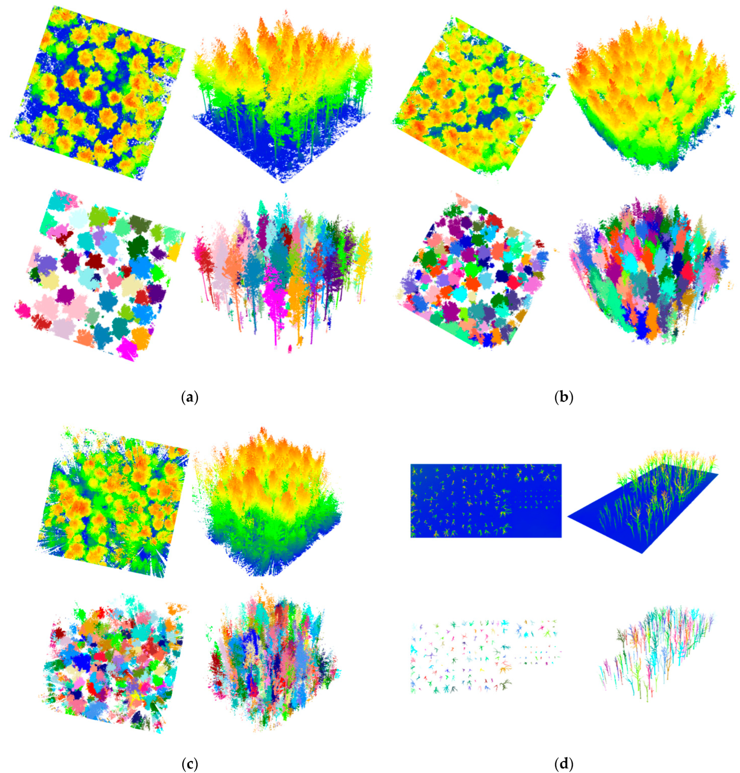
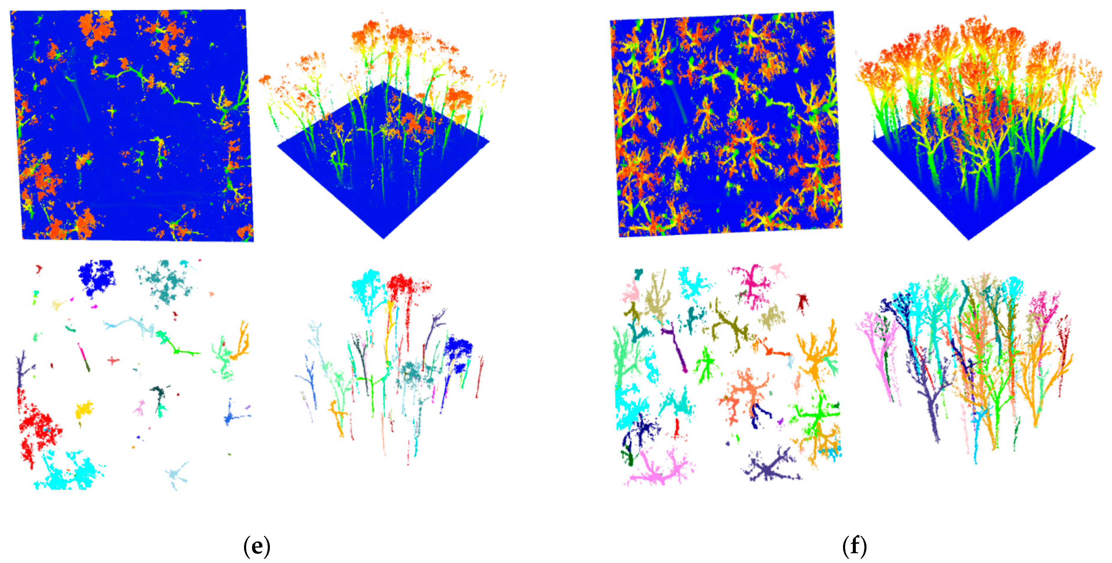
Examples of the segmentation results for each of the three difficulty levels present in the International TLS Benchmark dataset are shown in Figure 4a–c. As seen in Table 5, on this dataset our algorithm achieves a combined completeness score of 76%, correctness score of 79%, and IoU of 64%. Our algorithm outperforms the SOTA algorithm in completeness and IoU scores. The SOTA algorithm achieves a higher combined correctness score, indicating that segmented trees are more likely to be matched with a validation tree in the SOTA implementation. However, the SOTA algorithm only achieves a combined completeness score of 37%, indicating a high number of omissions. Taken together, these two metrics indicate that the SOTA implementation was only able to segment a few trees but found matches for most of the few trees it segmented.
We view completeness to be a more critical measure of performance than correctness. A low correctness value implies a high rate of commission errors (false positives) while a low completeness value implies a high rate of omissions (false negatives). While not desirable, commissions can be filtered out as a post-processing step if necessary. However, omissions cannot be recovered.
Reviewing the results from each International TLS Benchmark plot separately shows that our algorithm performs better than the SOTA in both completeness and IoU metrics regardless of scene complexity. Additionally, we observe a decrease in our algorithm’s performance as scene complexity increases. This is a trend found in nearly all tree segmentation methods, including the SOTA algorithm [15]. Our algorithm’s performance, however, decreases much less rapidly, significantly outperforming the SOTA in complex scenes. This is because our algorithm, unlike the SOTA, does not rely on the identification of trunk locations before segmentation. In complex scenes, the trunk is often hidden by brush or neighboring trees, making it difficult for trunks to be detected directly. Our algorithm avoids this source of error by finding trunks at the end of the segmentation process instead of making it a prerequisite.
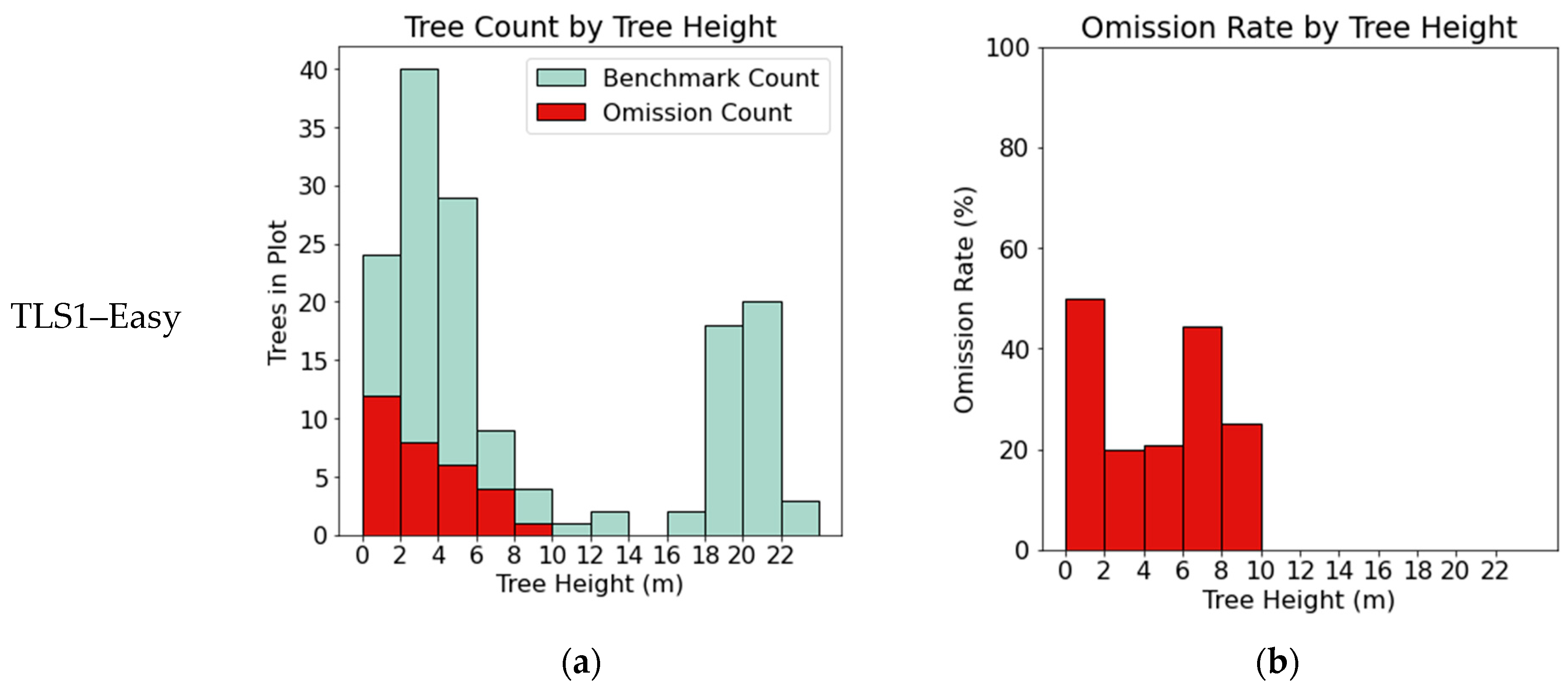
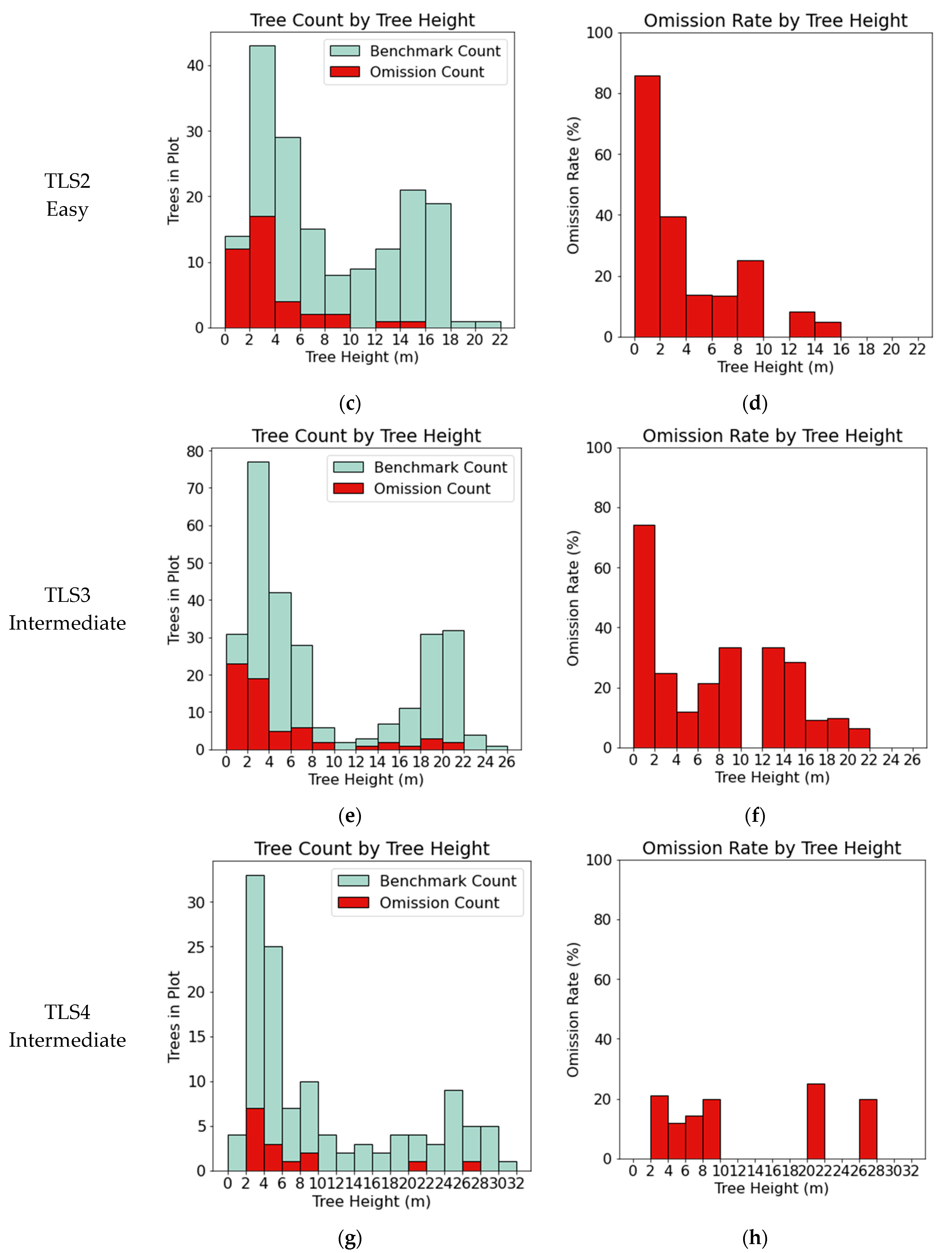
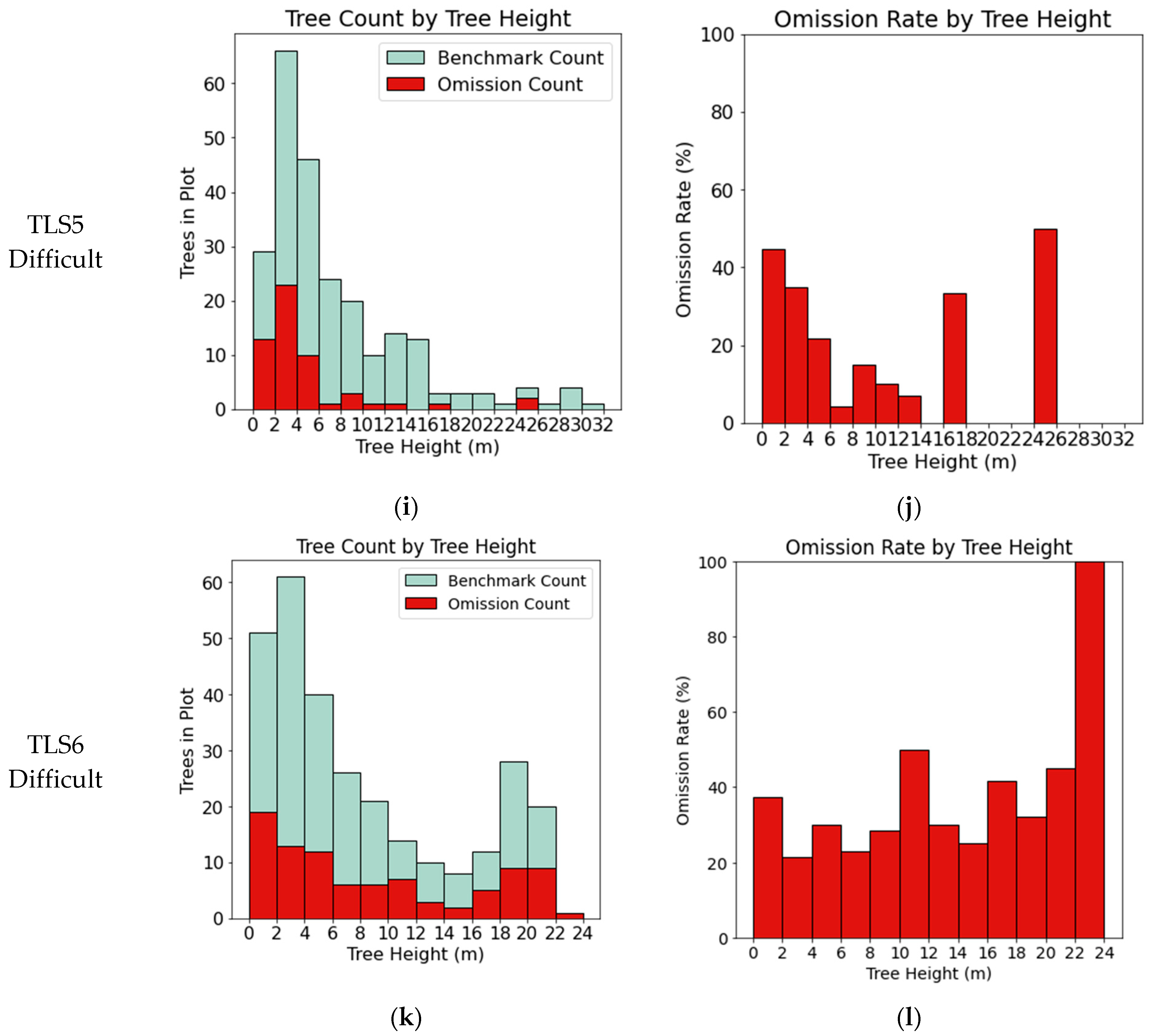
A significant difference between this paper and other papers which have used the International TLS Benchmarking dataset is the validation data used. Past work has only validated segmentation results on trees greater than 5 cm in diameter. This study digitized the positions and heights of all trees in the TLS datasets. This complete validation dataset allows omission errors to be analyzed by tree height. Figure 5a,b show the combined errors of omission from the six TLS datasets subdivided by validation tree height. While trees less than 4 m are omitted at a rate of 30–50%, taller trees have a lower omission rate of 15–20%. Figure A1 in the Appendix A contains the breakdown of omissions by tree height for each of the TLS datasets separately.
3.2. UAV-Based Photogrammetric Dataset
Two photogrammetric datasets were used for algorithm testing. Both were collected during leaf-off conditions. The first dataset, Photo-Plantation, was collected over a plantation of mature Walnut trees. This dataset is characterized by evenly spaced trees on a flat, mowed surface. This dataset achieved the best evaluation score (Table 6) with an IoU of 96%. The omission graphs (Figure 5c,d) show that the four omissions were of the smallest trees in the plot. Visual inspection of the point cloud reveals that these four trees were not captured by the input photogrammetrically constructed point cloud. The success of this plot is mainly due to the even spacing and well-maintained grounds present in the plot. The segmented point cloud can be viewed in Figure 4d.The second photogrammetric dataset, Photo-Natural, was captured over an area of natural forest. The raw point cloud and the segmented point cloud can be viewed in Figure 4e. Our algorithm performed better on this photogrammetric point cloud than on the UAV-based LiDAR dataset of the same stand. This is because photogrammetric reconstruction relies on finding single features in separate images. The automatic tie point algorithms used by Metashape rarely identify small features such as fine twigs or small branches in multiple images. This means that these features are not reconstructed. This artifact produces point clouds that contain none of the small vegetation noise common to both TLS datasets and UAV-based LiDAR. This demonstrates the advantage of using photogrammetry for tree stem mapping.
3.3. UAV-Based LiDAR Dataset
One UAV-based aerial LiDAR dataset was used for algorithm testing. LiDAR-Natural was collected over a naturally forested area with a lower-quality LiDAR unit. This dataset is characterized by a higher level of noise than the photogrammetric point clouds. This is caused firstly by the lower point precision achievable using the Zenmuse L1 and secondly because LiDAR will produce returns on small branches and fine vegetation. The extra noise in the dataset causes lower accuracy in the tree segmentation routine. This can be seen in the IoU value achieved, 53% (Table 6).
4. Discussion
4.1. Segmentation Error
Segmentation errors occur when our operating assumption—that the least-cost path from the canopy to the ground will route through the correct trunk—is invalid. There are three common cases when the assumption is invalid, and each causes a unique artifact in the segmentation results.
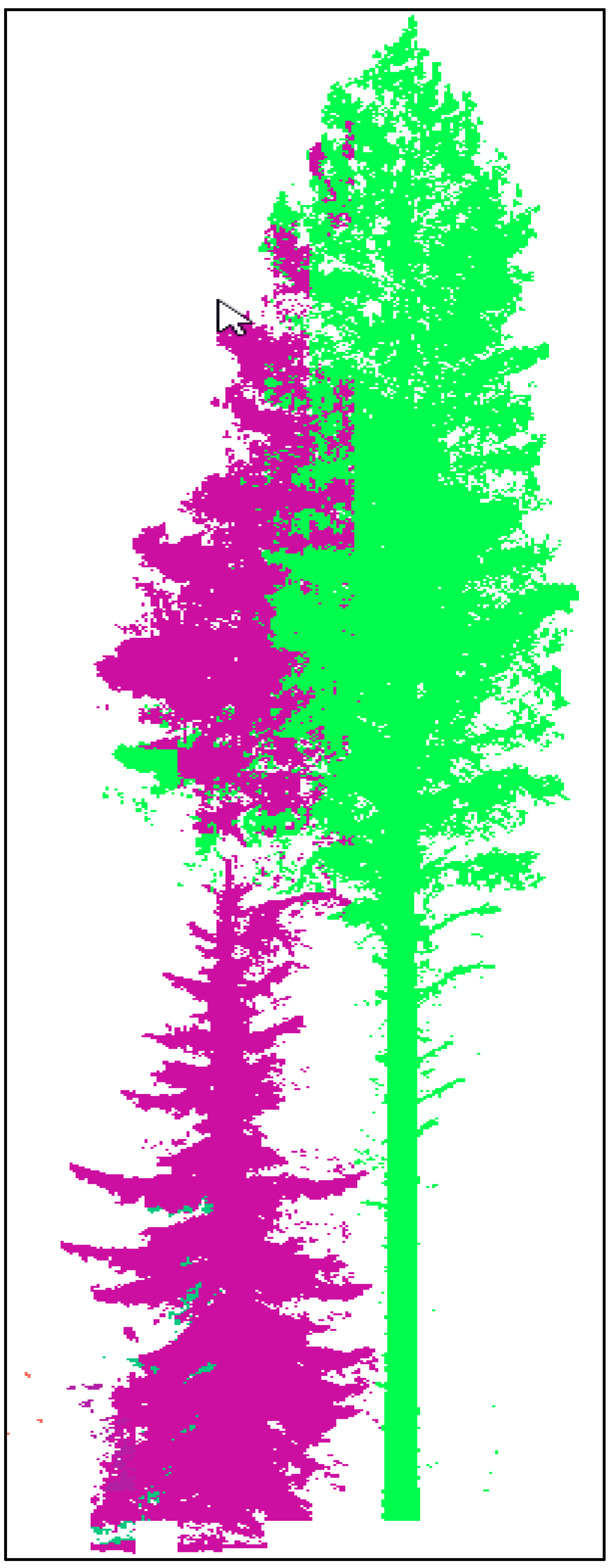
In case 1, a valid path from the canopy to the ground can be found through the branches, and not the trunk, of the tree. This causes the ‘split tree’ artifact as shown in Figure 6 This is often the case with coniferous trees where the branches are present along the entire length of the trunk or when grass or small trees grow thickly around the trunk of a deciduous tree. This case causes errors of commission because a single tree may be segmented into multiple trees.
Case 2 may not result in omissions or commissions but will result in a miss-segmentation of the point cloud. Called the ‘greedy tree’, this error arises when some portion of a tree’s canopy finds the lowest-cost path to the ground through a nearby tree. This error is especially prevalent in dense forests where several layers of the canopy are intertwined. An example is shown in Figure 7.
The ‘detached tree’ artifact occurs in case 3 because of data missing from the input point cloud (Figure 8). There are several causes of this missing data. In TLS data, occlusions from objects nearer to the scanner can cause trunks to be shadowed. In photogrammetric data, trees of small DBH are often missing from the point cloud after reconstruction. For any point cloud, errors from occlusions are much more prevalent in natural forests, as can be seen by the higher omission rates in the TLS, Photo-Natural, and LiDAR-Natural results when compared to the Photo-Plantation dataset. Missing data in the input dataset cannot be recreated by the proposed algorithm and will result in a missing or incorrectly segmented tree.
4.2. Canopy-to-Root Routing Direction
Past work which has used least-cost routing to segment individual trees has used a root-to-canopy direction for the routing algorithm. This direction necessitates dividing the segmentation process into two separate steps; first, the base of individual trees must be identified, then, least-cost routing can be used to attach the canopy points to individual roots. The work presented here recognizes that this process can be simplified into a single routing operation if the direction of routing is flipped. The proposed canopy-to-root method has allowed tree stem positions to be located and individual trees segmented without the need for a separate root-finding routine. The accuracy analysis shows that this simplification has not only matched published, state-of-the-art results, but has even exceeded state-of-the-art results on complex scenes.
As mentioned in the previous subsection, the major drawback of this method is its tendency to split single trees into multiple trees when vegetation or low-hanging branches obscure the trunk structure. This is particularly evident on coniferous trees, which tend to have larger branches lower on the trunk. In this case, routes traveling down from the canopy tend to diverge near the ground. Future work could focus on using a combination of canopy-to-root and root-to-canopy mapping to solve these problems. Canopy-to-root routing could find the trunks of deciduous trees, while a root-to-canopy direction could find coniferous trees.
4.3. Future Research
In addition to addressing the segmentation errors mentioned in Section 4.1, future research should also analyze the sensitivity of the segmentation results to the parameters, which are listed in Table 3. In this paper, the chosen values for the parameters were chosen through some trial and error and prior knowledge of the data.
5. Conclusions
Tree extraction and stem mapping are critical first steps in forest mapping and tree-scale feature extraction. The unsupervised canopy-to-root pathing (UCRP) routing presented here both segments the point cloud and discovers stem locations in a single routine. The proposed method was evaluated using six TLS benchmark datasets, two photogrammetric datasets collected during the leaf-off season, and one dataset collected from aerial LiDAR during the leaf-off season. Results show that we achieved state-of-the-art performances in individual segmentation and stem-mapping accuracy on the benchmark datasets. Additionally, our algorithm achieves similar performance on point clouds from photogrammetric reconstruction and aerial LiDAR sensors.
We anticipate the proposed segmentation approach to be added as an initial step in an automatic forest inventory pipeline. Since our algorithm performs well on both LiDAR and photogrammetry data modalities, we can support any type of large-area, high-resolution UAV mapping system. This provides a significant advance to 3d forest mapping and to the future of automatic forest inventory procedures.
Author Contributions
Conceptualization and methodology, J.C.; data curation, J.C., S.O. and B.H.; writing—original draft preparation, J.C.; writing—review and editing, J.J., S.O. and B.H.; supervision, J.J. and S.F.; funding acquisition, J.J. All authors have read and agreed to the published version of the manuscript.
Funding
This research is partially supported by the Purdue Integrated Digital Forestry Initiative.
Conflicts of Interest
The authors declare no conflict of interest.
Appendix A
Figure A1.
Omission errors for each of the 6 TLS data sets. Omission errors are aggregated by tree height. (a,c,e,g,i,k) show the number of omissions by tree height superimposed on the number of trees in the validation data of the same height class. (b,d,f,h,j,l) show the omission errors as a percentage of total trees within each height class.


References
- Raumonen, P.; Kaasalainen, M.; Åkerblom, M.; Kaasalainen, S.; Kaartinen, H.; Vastaranta, M.; Holopainen, M.; Disney, M.; Lewis, P. Fast Automatic Precision Tree Models from Terrestrial Laser Scanner Data. Remote Sens. 2013, 5, 491–520. [Google Scholar] [CrossRef]
- Yun, Z.; Zheng, G. Stratifying Forest Overstory and Understory for 3-D Segmentation Using Terrestrial Laser Scanning Data. IEEE J. Sel. Top. Appl. Earth Obs. Remote Sens. 2021, 14, 12114–12131. [Google Scholar] [CrossRef]
- Blackard, J.; Finco, M.; Helmer, E.; Holden, G.; Hoppus, M.; Jacobs, D.; Lister, A.; Moisen, G.; Nelson, M.; Riemann, R. Mapping U.S. Forest Biomass Using Nationwide Forest Inventory Data and Moderate Resolution Information. Remote Sens. Environ. 2008, 112, 1658–1677. [Google Scholar] [CrossRef]
- Vicari, M.B.; Disney, M.; Wilkes, P.; Burt, A.; Calders, K.; Woodgate, W. Leaf and Wood Classification Framework for Terrestrial LiDAR Point Clouds. Methods Ecol. Evol. 2019, 10, 680–694. [Google Scholar] [CrossRef]
- Peuhkurinen, J.; Maltamo, M.; Malinen, J.; Pitkänen, J.; Packalén, P. Preharvest Measurement of Marked Stands Using Airborne Laser Scanning. For. Sci. 2007, 53, 653–661. [Google Scholar]
- Wulder, M.; Niemann, K.O.; Goodenough, D.G. Local Maximum Filtering for the Extraction of Tree Locations and Basal Area from High Spatial Resolution Imagery. Remote Sens. Environ. 2000, 73, 103–114. [Google Scholar] [CrossRef]
- Zhao, K.; Popescu, S.; Nelson, R. Lidar Remote Sensing of Forest Biomass: A Scale-Invariant Estimation Approach Using Airborne Lasers. Remote Sens. Environ. 2009, 113, 182–196. [Google Scholar] [CrossRef]
- Pinz, A. A Computer Vision System for the Recognition of Trees in Aerial Photographs. Multisource Data Integr. Remote Sens. 1991, 3099, 111–124. [Google Scholar]
- Gougeon, F.A. A Crown-Following Approach to the Automatic Delineation of Individual Tree Crowns in High Spatial Resolution Aerial Images. Can. J. Remote Sens. 1995, 21, 274–284. [Google Scholar] [CrossRef]
- Culvenor, D.S. TIDA: An Algorithm for the Delineation of Tree Crowns in High Spatial Resolution Remotely Sensed Imagery. Comput. Geosci 2002, 28, 33–44. [Google Scholar] [CrossRef]
- Wang, L.; Gong, P.; Biging, G.S. Individual Tree-Crown Delineation and Treetop Detection in High-Spatial-Resolution Aerial Imagery. Photogramm. Eng. Remote Sens. 2004, 70, 351–357. [Google Scholar] [CrossRef]
- Gougeon, F.A.; Leckie, D.G. The Individual Tree Crown Approach Applied to Ikonos Images of a Coniferous Plantation Area. Photogramm. Eng. Remote Sens. 2006, 72, 1287–1297. [Google Scholar] [CrossRef]
- Ke, Y.; Quackenbush, L.J. A Review of Methods for Automatic Individual Tree-Crown Detection and Delineation from Passive Remote Sensing. Int. J. Remote Sens. 2011, 32, 4725–4747. [Google Scholar] [CrossRef]
- Lamar, W.R.; McGraw, J.B.; Warner, T.A. Multitemporal Censusing of a Population of Eastern Hemlock (Tsuga canadensis L.) from Remotely Sensed Imagery Using an Automated Segmentation and Reconciliation Procedure. Remote Sens. Environ. 2005, 94, 133–143. [Google Scholar] [CrossRef]
- Wang, D. Unsupervised Semantic and Instance Segmentation of Forest Point Clouds. ISPRS J. Photogramm. Remote Sens. 2020, 165, 86–97. [Google Scholar] [CrossRef]
- Westling, F.; Underwood, J.; Bryson, M. Graph-Based Methods for Analyzing Orchard Tree Structure Using Noisy Point Cloud Data. Comput. Electron. Agric. 2021, 187, 106270. [Google Scholar] [CrossRef]
- Hyyppä, E.; Yu, X.; Kaartinen, H.; Hakala, T.; Kukko, A.; Vastaranta, M.; Hyyppä, J. Comparison of Backpack, Handheld, Under-Canopy UAV, and Above-Canopy UAV Laser Scanning for Field Reference Data Collection in Boreal Forests. Remote Sens. 2020, 12, 3327. [Google Scholar] [CrossRef]
- Štroner, M.; Urban, R.; Línková, L. A New Method for UAV Lidar Precision Testing Used for the Evaluation of an Affordable DJI ZENMUSE L1 Scanner. Remote Sens. 2021, 13, 4811. [Google Scholar] [CrossRef]
- Liang, X.; Wang, Y.; Jaakkola, A.; Kukko, A.; Kaartinen, H.; Hyyppa, J.; Honkavaara, E.; Liu, J. Forest Data Collection Using Terrestrial Image-Based Point Clouds from a Handheld Camera Compared to Terrestrial and Personal Laser Scanning. IEEE Trans. Geosci. Remote Sens. 2015, 53, 5117–5132. [Google Scholar] [CrossRef]
- Roberts, J.; Koeser, A.; Abd-Elrahman, A.; Wilkinson, B.; Hansen, G.; Landry, S.; Perez, A. Mobile Terrestrial Photogrammetry for Street Tree Mapping and Measurements. Forests 2019, 10, 701. [Google Scholar] [CrossRef]
- Lisein, J.; Pierrot-Deseilligny, M.; Bonnet, S.; Lejeune, P. A Photogrammetric Workflow for the Creation of a Forest Canopy Height Model from Small Unmanned Aerial System Imagery. Forests 2013, 4, 922–944. [Google Scholar] [CrossRef]
- Carr, J.C.; Slyder, J.B. Individual Tree Segmentation from a Leaf-off Photogrammetric Point Cloud. Int. J. Remote Sens. 2018, 39, 5195–5210. [Google Scholar] [CrossRef]
- Fritz, A.; Kattenborn, T.; Koch, B. UAV-Based Photogrammetric Point Clouds- Tree Stem Mapping in Open Stands in Comparison to Terrestrial Laser Scanner Point Clouds. Int. Arch. Photogramm. Remote Sens. Spat. Inf. Sci. 2013, XL-1/W2, 141–146. [Google Scholar] [CrossRef]
- Liang, X.; Hyyppä, J.; Kaartinen, H.; Lehtomäki, M.; Pyörälä, J.; Pfeifer, N.; Holopainen, M.; Brolly, G.; Francesco, P.; Hackenberg, J.; et al. International Benchmarking of Terrestrial Laser Scanning Approaches for Forest Inventories. ISPRS J. Photogramm. Remote Sens. 2018, 144, 137–179. [Google Scholar] [CrossRef]
- Ben-Shabat, Y.; Lindenbaum, M.; Fischer, A. 3DmFV: Three-Dimensional Point Cloud Classification in Real-Time Using Convolutional Neural Networks. IEEE Robot. Autom. Lett. 2018, 3, 3145–3152. [Google Scholar] [CrossRef]
- Qi, C.R.; Su, H.; Mo, K.; Guibas, L.J. Pointnet: Deep Learning on Point Sets for 3d Classification and Segmentation. In Proceedings of the IEEE Conference on Computer Vision and Pattern Recognition, Honolulu, HI, USA, 21–26 July 2017; pp. 652–660. [Google Scholar]
- Mizoguchi, T.; Ishii, A.; Nakamura, H.; Inoue, T.; Takamatsu, H. Lidar-Based Individual Tree Species Classification Using Convolutional Neural Network. In Proceedings of the SPIE, Videometrics, Range Imaging, and Applications XIV, Munich, Germany, 26–27 June 2017; Volume 10332, pp. 193–199. [Google Scholar]
- Guan, H.; Yu, Y.; Ji, Z.; Li, J.; Zhang, Q. Deep Learning-Based Tree Classification Using Mobile LiDAR Data. Remote Sens. Lett. 2015, 6, 864–873. [Google Scholar] [CrossRef]
- Hamraz, H.; Jacobs, N.B.; Contreras, M.A.; Clark, C.H. Deep Learning for Conifer/Deciduous Classification of Airborne LiDAR 3D Point Clouds Representing Individual Trees. ISPRS J. Photogramm. Remote Sens. 2019, 158, 219–230. [Google Scholar] [CrossRef]
- Windrim, L.; Bryson, M. Detection, Segmentation, and Model Fitting of Individual Tree Stems from Airborne Laser Scanning of Forests Using Deep Learning. Remote Sens. 2020, 12, 1469. [Google Scholar] [CrossRef]
- Lin, Y.-C.; Liu, J.; Fei, S.; Habib, A. Leaf-Off and Leaf-On UAV LiDAR Surveys for Single-Tree Inventory in Forest Plantations. Drones 2021, 5, 115. [Google Scholar] [CrossRef]
- Sirmacek, B.; Lindenbergh, R. Automatic Classification of Trees From Laser Scanning Point Clouds. ISPRS Ann. Photogramm. Remote Sens. Spat. Inf. Sci. 2015, II-3/W5, 137–144. [Google Scholar] [CrossRef]
- Lin, Y.-C.; Habib, A. Quality Control and Crop Characterization Framework for Multi-Temporal UAV LiDAR Data over Mechanized Agricultural Fields. Remote Sens. Environ. 2021, 256, 112299. [Google Scholar] [CrossRef]
- Kuželka, K.; Slavík, M.; Surový, P. Very High Density Point Clouds from UAV Laser Scanning for Automatic Tree Stem Detection and Direct Diameter Measurement. Remote Sens. 2020, 12, 1236. [Google Scholar] [CrossRef] [Green Version]
- Itakura, K.; Hosoi, F. Automatic Individual Tree Detection and Canopy Segmentation from Three-Dimensional Point Cloud Images Obtained from Ground-Based Lidar. J. Agric. Meteorol. 2018, 74, 109–113. [Google Scholar] [CrossRef]
- Ayrey, E.; Fraver, S.; Kershaw, J.A.; Kenefic, L.S.; Hayes, D.; Weiskittel, A.R.; Roth, B.E. Layer Stacking: A Novel Algorithm for Individual Forest Tree Segmentation from LiDAR Point Clouds. Can. J. Remote Sens. 2017, 43, 16–27. [Google Scholar] [CrossRef]
- Zhang, W.; Wan, P.; Wang, T.; Cai, S.; Chen, Y.; Jin, X.; Yan, G. A Novel Approach for the Detection of Standing Tree Stems from Plot-Level Terrestrial Laser Scanning Data. Remote Sens. 2019, 11, 211. [Google Scholar] [CrossRef]
- Livny, Y.; Yan, F.; Olson, M.; Chen, B.; Zhang, H.; El-Sana, J. Automatic Reconstruction of Tree Skeletal Structures from Point Clouds. In Proceedings of the ACM SIGGRAPH Asia 2010 Papers on—SIGGRAPH ASIA ’10, Seoul, Korea, 15–18 December 2010; ACM Press: New York, NY, USA, 2010; p. 1. [Google Scholar]
- Neubert, B.; Franken, T.; Deussen, O. Approximate Image-Based Tree-Modeling Using Particle Flows. In Proceedings of the ACM SIGGRAPH 2007 Papers on—SIGGRAPH ’07, San Diego, CA, USA, 4–5 August 2007; ACM Press: New York, NY, USA, 2007; p. 88. [Google Scholar]
- Lin, Y.-C.; Shao, J.; Shin, S.-Y.; Saka, Z.; Joseph, M.; Manish, R.; Fei, S.; Habib, A. Comparative Analysis of Multi-Platform, Multi-Resolution, Multi-Temporal LiDAR Data for Forest Inventory. Remote Sens. 2022, 14, 649. [Google Scholar] [CrossRef]
- Hart, P.; Nilsson, N.; Raphael, B. A Formal Basis for the Heuristic Determination of Minimum Cost Paths. IEEE Trans. Syst. Sci. Cybern. 1968, 4, 100–107. [Google Scholar] [CrossRef]
- Wang, D. SSSC; GitHub Repository. 2020. Available online: https://github.com/dwang520/SSSC (accessed on 19 November 2021).
- Gale, D.; Shapley, L.S. College Admissions and the Stability of Marriage. Am. Math. Mon. 1962, 69, 9. [Google Scholar] [CrossRef]
Figure 1.
Cross-sections of the International TLS Benchmark datasets which demonstrate that the segmentation difficulty rating corelates with forest structure complexity. (a) ‘Easy’; (b) ‘Intermediate’; (c) ‘Difficult’. Points are colored based on relative height.
Figure 1.
Cross-sections of the International TLS Benchmark datasets which demonstrate that the segmentation difficulty rating corelates with forest structure complexity. (a) ‘Easy’; (b) ‘Intermediate’; (c) ‘Difficult’. Points are colored based on relative height.

Figure 2.
Map of Martell Forest, Indiana, USA. The red outline shows the forest’s boundaries. The yellow outlines show the location of the data collection sites.
Figure 2.
Map of Martell Forest, Indiana, USA. The red outline shows the forest’s boundaries. The yellow outlines show the location of the data collection sites.

Figure 3.
A 2D example showing the various stages of the of the tree segmentation algorithm presented in this paper. (a) The raw input point cloud. (b) The normalized input point cloud before superpoint encoding. (c) Visualization of the voxel divisions for superpoint encoding. (d) Results of superpoint encoding. (e) Results of rough classification. Red indicates ‘canopy’ superpoints, blue indicates ‘ground’ superpoints, and black indicates unlabeled superpoints. (f) Superpoints with a connectivity graph. In this toy example, k = 3. (g) Tree sets (distinguished by color) built by least-cost routing. (h) Three trees (blue, red, green, yellow) formed by grouping tree sets. (i) Mapping the tree labels back to the original point cloud points.

Figure 4.
Segmentation results for TLS, Photogrammetric, and LiDAR point clouds. In each tile, the top pair of images are different views of the raw point cloud colored by height and the bottom pair of images show the point cloud classified into individual trees. (a) An example of an ‘easy’ TLS plot. (b) An example of an ‘intermediate’ TLS plot. (c) An example of a ‘difficult’ TLS plot. (d) Photo-Plantation dataset. (e) Photo-Natural dataset. (f) LiDAR-Natural dataset.


Figure 5.
Omission errors are aggregated by tree height. (a,c,e,g) show the number of omissions by tree height superimposed on the number of trees in the validation data of the same height class. (b,d,f,h) show the omission errors as a percentage of total trees within each height class.
Figure 5.
Omission errors are aggregated by tree height. (a,c,e,g) show the number of omissions by tree height superimposed on the number of trees in the validation data of the same height class. (b,d,f,h) show the omission errors as a percentage of total trees within each height class.

Figure 6.
The ‘split tree’ error occurs when segmentation results split one tree into two because branches provide paths to the ground which do not route through the trunk.
Figure 6.
The ‘split tree’ error occurs when segmentation results split one tree into two because branches provide paths to the ground which do not route through the trunk.

Figure 7.
The ‘greedy tree’ artifact. The taller tree is segmented incorrectly because the shorter tree provides a route to the ground for the taller tree’s left side that does not pass through the taller tree’s trunk.
Figure 7.
The ‘greedy tree’ artifact. The taller tree is segmented incorrectly because the shorter tree provides a route to the ground for the taller tree’s left side that does not pass through the taller tree’s trunk.

Figure 8.
The ‘detached tree’ artifact. Two trees are segmented as a single tree because the trunk of the right tree is missing from the data.
Figure 8.
The ‘detached tree’ artifact. Two trees are segmented as a single tree because the trunk of the right tree is missing from the data.


Table 1.
The flight parameters of the UAV LiDAR mission.
| LiDAR-Natural | |
|---|---|
| Altitude | 100 m |
| Lidar Pulse Rate | 240 kHz |
| Flying Speed | 6 m/s |
| Sidelap | 80% |
Table 2.
The flight parameters of the UAV Photogrammetry missions.
| Photo-Plantation | Photo-Natural | |
|---|---|---|
| Altitude | 80 m | 110 m |
| Ground Sampling Distance | 1 cm | 1.4 cm |
| Overlap | 90% | 90% |
| Sidelap | 90% | 80% |
Table 3.
A list of the user-defined parameters used in the proposed algorithm.
| Symbol | Description | Value in This Paper |
|---|---|---|
| Size of the voxel cube used to compute superpoints | 0.3 m | |
| A voxel must contain more than points to be used to create a super point | 10–TLS and Photo Datasets 2–LiDAR Dataset | |
| A threshold value determining the highest elevation for a ‘ground’-classified superpoint | 1.2 m | |
| A threshold value determining the lowest elevation for a ‘canopy’ superpoint | 2 m | |
| The number of nearest neighbors connected to each superpoint in the initial graph construction | 10 | |
| The merge distance within which two tree sets will be merged to form a single tree | 0.9 m |
Table 4.
Parameter values used in the SOTA implementation.
| Parameter | Value |
|---|---|
| Threshold | 0.125 |
| Height | Ranged from 2–10 |
| NoP | 100 |
| Verticality | Ranged from 0.6–0.8 |
| Length | 2 |
| Merge Range | 0.3 |
Table 5.
Tabulated segmentation results achieved by our UCRP algorithm, and comparison of our algorithm and the SOTA algorithm [15] on the International TLS Benchmarking Datasets. Bold indicates the best performer.
Table 5.
Tabulated segmentation results achieved by our UCRP algorithm, and comparison of our algorithm and the SOTA algorithm [15] on the International TLS Benchmarking Datasets. Bold indicates the best performer.
| Dataset | Reference Trees | Segmented Trees | Matched Trees | Omissions | Commissions | Completeness% | Correctness % | IoU % | |||
|---|---|---|---|---|---|---|---|---|---|---|---|
| Ours | Wang | Ours | Wang | Ours | Wang | ||||||
| TLS1–Easy | 152 | 139 | 121 | 31 | 18 | 79 | 38 | 87 | 93 | 71 | 37 |
| TLS2–Easy | 172 | 137 | 133 | 39 | 4 | 77 | 38 | 97 | 94 | 75 | 37 |
| TLS3–Intermediate | 275 | 256 | 211 | 64 | 45 | 76 | 50 | 82 | 93 | 65 | 48 |
| TLS4–Intermediate | 121 | 168 | 106 | 15 | 62 | 87 | 23 | 63 | 76 | 57 | 22 |
| TLS5–Difficult | 242 | 256 | 187 | 55 | 69 | 77 | 55 | 73 | 83 | 60 | 50 |
| TLS6–Difficult | 292 | 256 | 200 | 92 | 56 | 68 | 1 | 78 | 80 | 57 | 1 |
| Totals | 1254 | 1212 | 958 | 296 | 254 | 76 | 37 | 79 | 90 | 64 | 36 |
Table 6.
Tabulated segmentation results achieved by our UCRP algorithm, and comparison of our algorithm to the SOTA algorithm [15] on the Photogrammetry and LiDAR Datasets. Bold indicates the best performer.
Table 6.
Tabulated segmentation results achieved by our UCRP algorithm, and comparison of our algorithm to the SOTA algorithm [15] on the Photogrammetry and LiDAR Datasets. Bold indicates the best performer.
| Dataset | Reference Trees | Segmented Trees | Matched Trees | Omissions | Commissions | Completeness% | Correctness % | IoU % | |||
|---|---|---|---|---|---|---|---|---|---|---|---|
| Ours | Wang | Ours | Wang | Ours | Wang | ||||||
| Photo–Plant. | 133 | 129 | 129 | 4 | 0 | 96 | 54 | 100 | 96 | 96 | 52 |
| Photo–Natural | 51 | 54 | 44 | 7 | 10 | 86 | 25 | 81 | 84 | 72 | 24 |
| LiDAR–Natural | 71 | 49 | 42 | 29 | 7 | 59 | 15 | 85 | 83 | 53 | 15 |
Publisher’s Note: MDPI stays neutral with regard to jurisdictional claims in published maps and institutional affiliations. |
© 2022 by the authors. Licensee MDPI, Basel, Switzerland. This article is an open access article distributed under the terms and conditions of the Creative Commons Attribution (CC BY) license (https://creativecommons.org/licenses/by/4.0/).
Share and Cite
MDPI and ACS Style
Carpenter, J.; Jung, J.; Oh, S.; Hardiman, B.; Fei, S. An Unsupervised Canopy-to-Root Pathing (UCRP) Tree Segmentation Algorithm for Automatic Forest Mapping. Remote Sens. 2022, 14, 4274. https://doi.org/10.3390/rs14174274
AMA Style
Carpenter J, Jung J, Oh S, Hardiman B, Fei S. An Unsupervised Canopy-to-Root Pathing (UCRP) Tree Segmentation Algorithm for Automatic Forest Mapping. Remote Sensing. 2022; 14(17):4274. https://doi.org/10.3390/rs14174274
Chicago/Turabian StyleCarpenter, Joshua, Jinha Jung, Sungchan Oh, Brady Hardiman, and Songlin Fei. 2022. "An Unsupervised Canopy-to-Root Pathing (UCRP) Tree Segmentation Algorithm for Automatic Forest Mapping" Remote Sensing 14, no. 17: 4274. https://doi.org/10.3390/rs14174274
Note that from the first issue of 2016, this journal uses article numbers instead of page numbers. See further details here.