Using Process Based Snow Modeling and Lidar to Predict the Effects of Forest Thinning on the Northern Sierra Nevada Snowpack

Introduction

Upland snowmelt is a vital water resource for downstream populations and local ecological systems. Snow is particularly important in regions with Mediterranean climates, such as the Sierra Nevada in the western US, where snowmelt provides the majority of the water supply. Increasing temperatures in such regions are shortening the snow accumulation season, increasing the frequency of mid-winter snowmelt events and producing earlier snowmelt runoff (López-Moreno et al., 2013; Musselman et al., 2017a; Harpold and Brooks, 2018; Mote et al., 2018), with significant ecological and economic impacts (Sturm et al., 2017). Tree removal, and particularly targeted forest thinning, has the potential to increase snow accumulation and melt through a reduction in snowfall that is intercepted and sublimated from forest canopy (Varhola et al., 2010; Tague et al., 2019). However, there is significant regional variability in the snowpack response to tree removal due to differences in climate, topography, forest species, and the spatial distribution of trees on the landscape (Varhola et al., 2010). Key snow processes are highly sensitive to forest canopy, such as snowpack sublimation, blowing snow redistribution, incoming radiation, and turbulent energy fluxes (Anderson et al., 1976; Troendle and Leaf, 1980; Golding and Swanson, 1986; Toews and Gluns, 1986; Pomeroy and Granger, 1997; Pomeroy et al., 2002; Winkler et al., 2005; Bewley et al., 2010). Early studies in the Sierra Nevada, California, have shown that forest patches with glades accumulate more snow than dense forest patches (Church, 1933; Anderson, 1956, 1963), consistent with the idea that tree removal increases snowmelt volume. However, it remains challenging to quantify the response of the snowpack's mass and energy budgets to tree removal over relatively large domains (e.g., >10 km²). Large domain simulations that capture key fine-scale processes are needed to predict hydrologic responses to forest restoration efforts, which span substantial gradients of climate, topography, and vegetation removal.

Paired watershed experiments and studies comparing canopy clearings with under canopy locations have provided insights into the effect of forest removal on snow processes (Anderson et al., 1976; Troendle and Leaf, 1980; Alexander et al., 1985; Golding and Swanson, 1986; Toews and Gluns, 1986; Pomeroy et al., 2002; Woods et al., 2006). However, many of these studies are constrained by relatively small domains (e.g., Goodell, 1952) that limit their scalability and representativeness for larger domains with more variable vegetation and topographic conditions. Model predictions of snowpack response typically use spatially-averaged parameters to represent snow-forest interactions (Essery et al., 2009; Rutter et al., 2009) that fail to represent the spatial heterogeneity of forests. A lack of model fidelity can be problematic because snow processes do not vary linearly across spatial scales (Blöschl, 1999). Current modeling approaches are likely to provide biased estimates of the effect of forest thinning on snowpack at large scales. For example, Broxton et al. (2015) found that coarsening the spatial resolution of a process-based snow model from 1 to 100 m reduced peak snow water equivalent (SWE) between 14 and 24% due to the simplification of radiation transfer processes. These types of studies demonstrate the importance of tree-scale processes to make accurate snowpack predictions of heterogeneous forest change.

Increasing availability of aerial light detection and ranging (lidar) datasets from snow-covered forests, combined with improved computational resources, has the potential to revolutionize model representations of small-scale snow-forest interactions (Moeser et al., 2014, 2015; Musselman et al., 2015, 2017b). Very high spatial resolution models (e.g., 1 m) allow a spatially explicit representation of heterogeneous forest canopy and associated snowpack processes (Broxton et al., 2015; Moeser et al., 2015). However, applications of these models using lidar are rare due to computational requirements and issues related to model development, calibration, and validation. One of the first efforts to develop a full energy budget snowmelt model at high resolution was Broxton et al. (2015), who created the Snow Physics and Lidar Mapping (SnowPALM) model, which uses lidar data to parameterize vegetation structure. Broxton et al. (2015) successfully validated SnowPALM using both snow pillow data and lidar-derived snow depths at two sites in the central and southern Rocky Mountains. Harpold et al. (2020) extended the application of SnowPALM to the Sierra Nevada, California, and developed new validation datasets of snow depth and surface temperature across different forest structures. Their study investigated the effects of a “virtual thinning” on snow mass and energy fluxes over a relatively small domain (1,200 × 1,200 m), and showed which forest and topographic conditions had the greatest increases in snowmelt volume after removing trees of different heights. However, there remains uncertainty about snowpack response to forest thinning over large areas and a lack of detailed recommendations needed for ongoing forest restoration efforts.

Building upon this recent work, we extend this high-resolution SnowPALM modeling to a much larger domain encompassing two medium sized (~25 km² each) mountain watersheds on the west shore of Lake Tahoe, California. These watersheds are part of the Lake Tahoe West Restoration Partnership, which aims to develop a landscape restoration strategy that increases the resiliency of this region to drought, climate change, and extreme fire. Tree (fuel) removal is a common fire suppression practice in this region; however, its impact on snow accumulation and melt volumes are not considered as part of the thinning strategies. This study was developed as an effort to provide actionable scientific information to forest and water managers in the region, along with a decision support tool that can be readily deployed with relatively few computational resources. For this purpose, we parameterized the SnowPALM model to predict snowpack response to two “virtual thinning” scenarios where all trees below 10 and 20-m tall were removed. We then used these simulations to train a machine-learning algorithm that informs a decision support tool for forest managers to determine where thinning should be performed. These simulations were used to answer four questions: (1) which tree removal scenario provides the largest increases in snow accumulation and melt volumes? (2) what are the characteristics of forest stands that yield the greatest water benefits from thinning and what is their topographic distribution? (3) what are the physical mechanisms that explain this variation in snow water benefits from thinning and how do they vary over topography? and (4) can we develop a decision support tool that synthesizes high resolution modeling to extract more information from the models about best thinning practices within and outside of the study area?

Study Site

Two mountainous watersheds along the west shore of Lake Tahoe (Figure 1) in California were chosen for this study because they represent a large variation in topography and vegetation, and have detailed hydrological observations: Ward Creek (24.9 km²) and Blackwood Creek (28.9 km²). Elevation ranges from roughly 1,900 masl at the shore of Lake Tahoe, which has gentle slopes and tall and dense forest, to 2,700 masl where much steeper and sparsely vegetated slopes exist. These two watersheds have high resolution (1 m) lidar estimates of vegetation height and density (Xu et al., 2018), as well as snow depth and SWE measurements from Snow Telemetry (SNOTEL) stations within and nearby these watersheds. This region has a Mediterranean-type climate with dry, hot summers and wet winters. The 30-year climate normal (1980–2010) from the nearby Tahoe City weather station (from the US National Weather Service) shows a mean annual air temperature of 6.4°C and a maximum and minimum mean monthly air temperature of about 16 and −7°C in July and January, respectively. Mean annual precipitation for the same period is estimated to be 870 mm, from which about 78% falls during November and March. Snow accumulation at the SNOTEL station in Ward Creek (Figure 1) typically starts in early November and lasts until mid-May. Tree species in the Tahoe Basin consist predominantly of Jeffrey Pine (pinus Jeffrey balf.), Ponderosa Pine (pinus pondersa), Red Fir (abies magnifica), Lodgepole Pine (pinus contorta), and White Fir (abies concolor) (van Gunst, 2012).

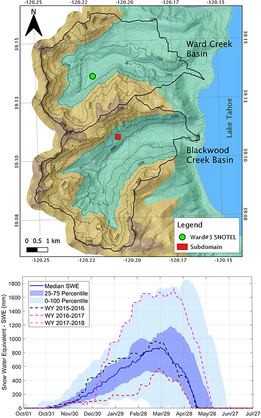
Figure 1. Upper panel: Relief map showing the modeled basins along the west shore of Lake Tahoe, California (contour interval = 100 m). The red rectangle shows the subdomain (150 × 150 m) presented in Figure 4. Lower panel: Observed snow water equivalent (SWE) climatology at the Ward #3 SNOTEL station, including the observed SWE for the three water years simulated in this study (dashed lines).

Methods

Snow Modeling

The Snow Physics and Lidar Mapping (SnowPALM; Broxton et al., 2015) model was used to simulate the mass and energy budgets of snow in forested areas with complex topography. Broxton et al. (2015) describes SnowPALM parameterization and model development; however, key features are also presented here. SnowPALM simulates snow processes at a high spatial (1 m) and temporal (1 h) resolution, which is particularly important for applications in regions with complex terrain and heterogeneous forest structure, as it improves the model's fidelity to simulate snow-forest interactions. SnowPALM simulates snowpack using a one-layer snow energy and mass balance whose skin temperature is calculated separately through an energy balance between net radiation, sensible heat and heat conduction to the middle of the snowpack and a one-layer soil to compute ground heat exchange. SnowPALM also simulates wind distribution of snowfall (Winstral and Marks, 2002), canopy interception and evaporation/sublimation of rainfall/snowfall, canopy unloading of rain/snow (Deardorff, 1978; Pomeroy et al., 1998), attenuation of shortwave radiation by the canopy (Mahat and Tarboton, 2012), longwave radiation from the forest (whose skin temperature is calculated balancing net radiation with turbulent fluxes assuming a snow-free canopy albedo), and albedo decay as a function of time. The liquid water that falls on top of the snowpack, either from rain passing through the canopy or canopy drip, can either freeze to the snowpack or pass through the snowpack and infiltrate into the soil. Hereafter, we will refer to the sum of this infiltrated water and snowmelt as “net water input,” or the total water emanating from the snowpack that is available for infiltration and runoff.

The meteorological data used in this study are from phase 2 of the North American Land Data Assimilation System (NLDAS-2; Xia et al., 2012), which provides hourly precipitation, air temperature, wind speed and direction, air pressure, downward shortwave and longwave radiation, and specific humidity at 1/8 of degree spatial resolution. These data were downscaled using SnowPALM's built-in downscaling procedures, using a combination of linear interpolation (for some variables) and relationships with elevation derived from the Parameter-elevation Regressions on Independent Slopes Model (PRISM) monthly maximum/minimum temperature and precipitation data. Three water years (starting in October 1) were simulated in this study: 2015–2016, 2016–2017, and 2017–2018, hereafter referred as WY16, WY17, and WY18, respectively. These years represent a wide range of historical conditions, ranging from relatively dry (WY18), normal (WY16), and wet (WY17) conditions (lower panel Figure 1).

The model parameterization used in this study is the same as the one presented by Harpold et al. (2020), who used data from three different SNOTEL stations: Rubicon#2 (ID: 724, about 15 km south of Ward Creek), Ward Creek#3 (ID: 848) and Tahoe City Cross (ID: 809, about four km north of Ward Creek) for calibration and validation. The idea behind this cross-site calibration/validation was to produce a model capable of representing the snowpack at more than a single location to reduce the uncertainty of parameter estimation. However, emphasis was given to representing snowpack conditions at the Rubicon#2 SNOTEL station, which is located within their study domain. Key parameters adjusted in SnowPALM during calibration relate to reduction of biases in the gridded forcing data and a parameter describing the leaf area index (LAI) of fully dense canopy. For a detailed description of the parameterization used in the model, the readers are referred to Harpold et al. (2020).

Lidar Datasets and Virtual Thinning Experiments

Airborne lidar was collected for an area surrounding Lake Tahoe from August 11 and 24, 2010 (Romsos, 2011). The average first return point density was 11.82 point/m², the average ground point density was 2.26 point/m², and the vertical accuracy (RMSE) was estimated to be 3.5 cm. The point cloud dataset was downloaded from OpenTopography.org (http://opentopo.sdsc.edu/datasetMetadata?otCollectionID=OT.032011.26910.1, accessed October 1, 2019) in LAS 1.4 format. Vegetation height, density, and leaf area index (LAI) were derived from the lidar point cloud and a bare-earth model (from OpenTopography) to parameterize SnowPALM. Vegetation height was calculated as the difference between the canopy height model and the bare-earth model at 1 m resolution. Canopy density was computed as the ratio between non-ground return (>2 m above the ground surface) and total returns per square meter. LAI at 1-m resolution was defined as the product of vegetation density and an estimated maximum LAI of 4 m²/m², based on the local observation presented by van Gunst (2012).

Two virtual thinning scenarios were created, following the thinning experiment presented by Harpold et al. (2020). These scenarios consist of removing all trees <10 and 20-m tall, which are considered to be scenarios of moderate and significant forest disturbance, respectively. These were created by changing LAI and vegetation height to zero for all the pixels with vegetation height below 10 and 20 m using the tree-delineated dataset from Xu et al. (2018). This type of forest disturbance was selected to mimic forest management strategies in the region, which are primarily design to reduce the risk of severe forest fires while maintaining the recreational and aesthetic value of the forest. SnowPALM was run for the Ward Creek and Blackwood Creek Basins, using maps generated for these two thinning scenarios (10 and 20 m removal simulations) and those representing the current forest conditions (control run).

To understand the impact of the two virtual thinning experiments on the snowpack across a large topographic gradient, the modeling domain was divided into five ~160-m elevation bands (low, mid-low, mid, mid-high, and high), and north and south facing aspects, resulting in 10 regions that we termed “Snow Zones.” The high elevation Snow Zones are steeper (average slope ~40%) than those at lower elevations (average slope ~20%, Figure 2). Low elevation Snow Zones also have denser and taller trees than high elevation Snow Zones (Figure 2), where mean tree height and density include non-vegetated areas. Peak SWE at low elevations is less than half of that at high elevations and the snow lasts about 45 days longer at high elevations (Figure 2). Snow disappearance is 2–3 weeks later on the north-facing Snow Zones compared to south-facing Snow Zones with the same elevation (Figure 2). The 1-m SnowPALM simulations were averaged to 30-m grids to investigate the effect of forest thinning on the snowpack at a meaningful scale for forest managers.

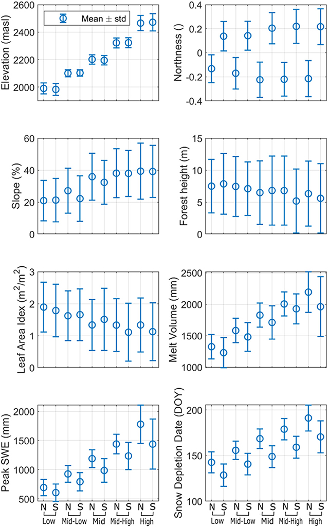
Figure 2. Mean (± standard deviation) Snow Zones' topography, vegetation and snow conditions for the water years 2016–2018 as simulated by SnowPALM. Values for forest LAI and height include non-vegetated areas within each Snow Zone. “N” and “S” on the x-axis represent north- and south-facing Snow Zones.

Random Forest (RF) Decision Support Tool

The goal of the decision support tool is to extend our findings to areas outside the SnowPALM modeling domain and to identify priority management areas where forest thinning is likely to have the most positive benefits for water supply. We used a regression-type of Random Forest (Breiman, 2001) (RF) algorithm to learn from the SnowPALM simulations. The RF was developed to predict how changes in forest structure affect snowpack under a wide range of topographic (e.g., north vs. south facing slopes) and climatic (e.g., warm and cold) conditions. RF models have a strong track record in snow hydrology and have been previously used to understand the spatial distribution of the snowpack using lidar (Tinkham et al., 2014) and fractional snow cover (Petersky et al., 2018). In this application, RF is used to predict 30-m changes to total net water input using the following predictors: elevation, aspect, slope, existing forest height and LAI, and changes to forest LAI (between the existing forest and the virtual thinning scenarios). It was implemented using the function TreeBagger in Matlab^®. This function uses a bootstrapping algorithm to sample the data and train each tree. At each decision split or “branch,” the algorithm selects a random subset of predictors to be used in the regression tree. Ultimately, it combines the results of all decision trees to predict a response, reducing problems with overfitting the training dataset. We used 50 trees in the RF as this converged to a minimum “out-of-bag” error. The out-of-bag error is the error when using the dataset not selected by the bootstrapping algorithm to run the RF, similar to a cross-validation. An importance metric for each predictor was calculated using the out-of-bag dataset, where each predictor (e.g., elevation) was randomly permuted (one at a time) and used to run the RF. The predictions from these runs were then compared to those using the original out-of-bag dataset to compute the importance metric. Predictors with higher errors after the random permutation were the most “important” (i.e., sensitive) in the RF.

Results

SnowPALM Validation

Harpold et al. (2020) showed SnowPALM's good performance against observed SWE and snow depth at the Rubicon #2 SNOTEL, consisting of a snow pillow in a forest clearing. They also showed the model's adequate performance against snow surface temperature and depth under different canopy conditions. Here, we compare snow observations from the other two SNOTEL sites in the region (Tahoe City Cross and Ward Creek SNOTELs) against SnowPALM simulations. The SWE comparison is at the snow pillow scale, where the 1-m SWE simulations are averaged to match the extent of the snow pillow on the ground. The model generally captures the accumulation season relatively well for the different water years and across sites. However, during the wet WY17, peak SWE at Ward Creek #3 is overestimated by 350 mm (20%), whereas at Tahoe City Cross, it is underestimated by 156 mm (25%). These differences are related to difficulties representing how air temperature influences precipitation phase at each SNOTEL site using the NLDAS-2 (and PRISM) data. For example, at Ward Creek #3, air temperature during the period of peak SWE was underestimated (Figure 3), resulting in some rainfall events being simulated as snowfall, leading to an overestimation of peak SWE. Despite the imperfect match against SNOTEL data, the validation is strong and consistent with previous studies (Harpold et al., 2020). Although this study lacks of detailed in situ measurements to validate SnowPALM, Harpold et al. (2020) validated SnowPALM using snow depth and snow surface temperature observations in open and under canopy environments on a nearby site (15 km south) with similar physiographic conditions, showing an adequate model performance. Furthermore, Broxton et al. (2015) showed a detailed lidar-based validation of SnowPALM in the mountains of Colorado and New Mexico under different degrees of canopy cover, demonstrating its ability to reproduce the effect of canopy on snow accumulation and melt. Moreover, this study does not require a perfect match at all sites because it analyzes the relative differences of snowpack between the modeling scenarios.

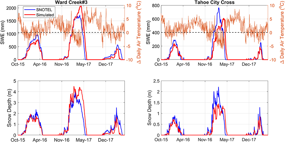
Figure 3. Model validation of snow water equivalent (SWE) and snow depth for Ward #3 (Left) and Tahoe City Cross (Right) SNOTEL stations. Upper panels include the difference between simulated and observed mean daily air temperature, with positive values indicating a model overestimation.

Example of Forest Thinning at 1-m Spatial Resolution

Figure 4 shows 1-m differences between snowpack simulations for the 20-m thinning scenario and the control run at a relatively low elevation and north-facing subdomain (150 × 150 m, Figure 1). Overall, across this subdomain, melt volume increases by 14% on average, with substantial variability. Some areas show increases up to 80%, while other areas with little tree cover show a decrease in melt volume and peak SWE. Thinning decreased the total canopy sublimation by 130 mm on average (including areas without changes), with some decreases ranging up to 400 mm. Changes to snowpack sublimation, which depend on changes to the incoming net radiation (shortwave and longwave radiation), the wind regime, and the duration of the snowpack, are relatively small and variable across the domain. Net incoming radiation increased in most places where trees were removed due to increased solar exposure after thinning; however, some areas near previously existing (but removed) warm trees that emitted large amounts of longwave radiation show a decrease. Areas showing decreases in net radiation are found at the south edges of existing tree stands in relatively open areas (upper left and right areas of the subdomain). Overall, changes to peak SWE and net water input reflect complex interactions between mass and energy fluxes.

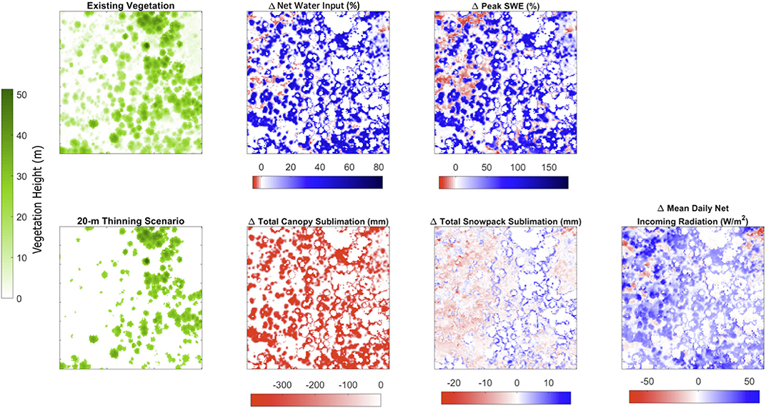
Figure 4. Subdomain (150 × 150 m; see red box in Figure 1) example at 1-m resolution for the 20-m thinning scenario in the WY16. Left panels show pre- and post-thinning vegetation height, and the remaining panels show changes (thinning scenario—control run) in net water input, peak SWE, total canopy sublimation, total snowpack sublimation, and average incoming solar radiation during the snow covered season.

Impacts of Forest Thinning Across Snow Zones on Mass and Energy Fluxes

When thinning results are aggregated to the 30-m scale (forest patch) to better match scales where management decision are made, there is a strong positive linear relationship between changes of LAI and changes of net water input for all Snow Zones (Figure 5; r² from 0.76 to 0.95 and RMSE from 16 to 42 mm). The slopes of the linear relationships suggest that melt volume changes in mid to mid-low elevation Snow Zones are most sensitive to changes in canopy cover (slopes between 121 and 125 mm/m²m⁻²), whereas at high elevations, net water input changes are about 10% less sensitive (slope <107 mm/m² m⁻²). Scatter plots between canopy cover changes and peak SWE are similar to those for net water input (Supplementary Figure 1); however, lower correlations and steeper slopes are found in mid- to high-elevation Snow Zones. These relationships not only show the importance of absolute forest removal to changes in melt volume and peak SWE (i.e., strength of linear relationships), but also that forest thinning of the same magnitude may have uneven results (note the scatter in Figure 5 and Supplementary Figure 1).

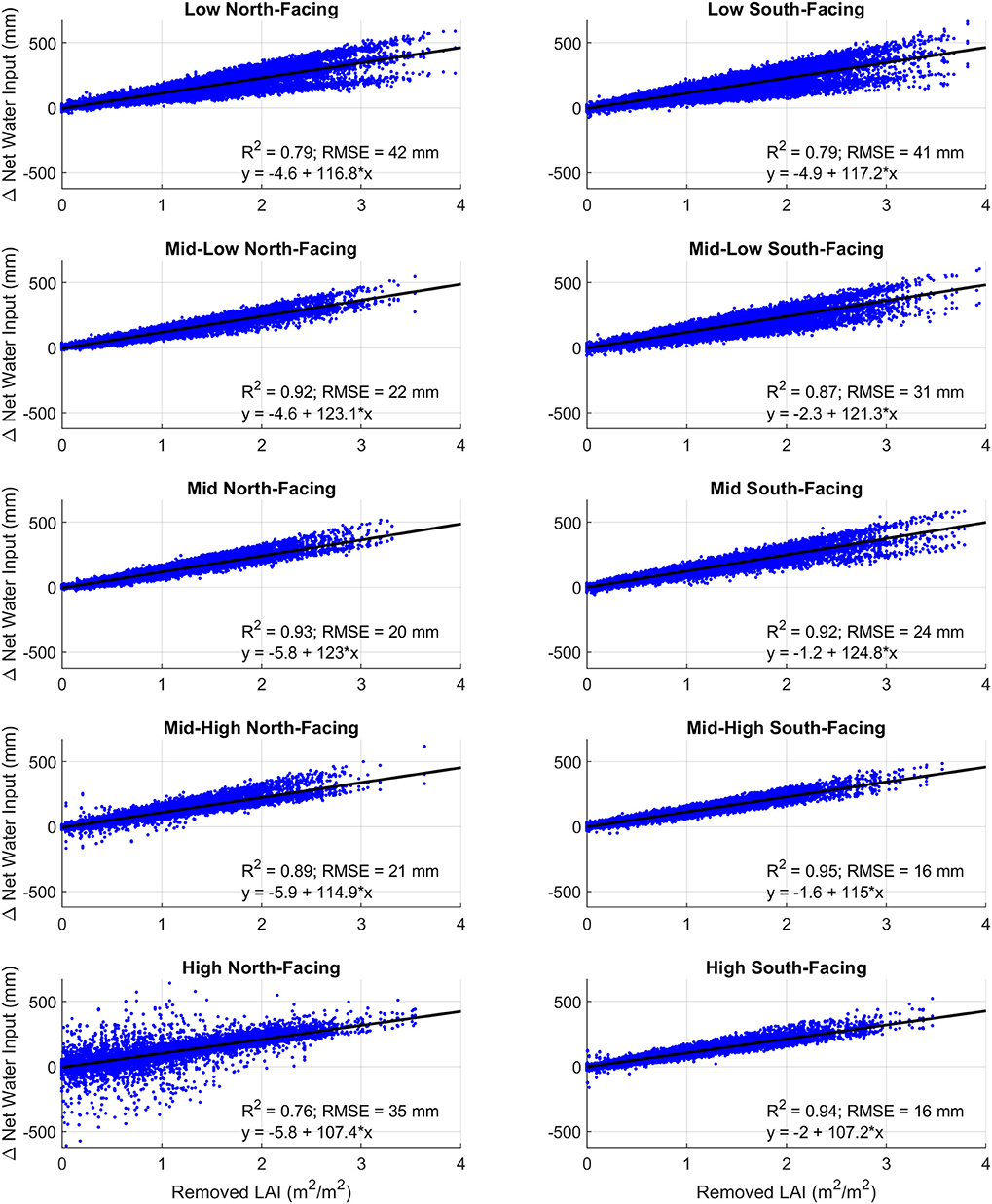
Figure 5. Forest patch (30 m) relationships between changes in net water input and removed LAI for the two thinning scenarios and the three water years across Snow Zones.

To identify which 30-m forest patches have the largest increases in net water input and peak SWE in response to forest thinning, we investigate these changes in relation to their forest structure prior to thinning (Figures 6, 7). Snow Zones that show the largest increases in net water input (i.e., >500 mm) are the Low North, Low South, Mid-Low South, and Mid South Snow Zones (Figure 6 and Supplementary Figure 11). Forest patches that have the largest increase in net water input from tree removal are those that are relatively dense (LAI > 3 m²/m²) with an average forest height of 5–15 m (Figure 6). Forest patches with those characteristics typically have many trees (stem density >50) with mean height up to roughly 30 m (Supplementary Figure 2), resulting in scattered tall trees after thinning. Forest patches with this vegetation structure provide the largest decrease of canopy sublimation (Supplementary Figure 3) and relatively low increase in incoming net radiation (Supplementary Figure 4), resulting in the largest increase in melt volume. Large net water input increases (>500 mm) also occur for a few forest patches with low LAI (<2 m²/m²) and canopy height (<5 m) in the High North Snow Zone. These increases are not caused by changes to canopy sublimation (Supplementary Figure 3) or snowpack sublimation (Supplementary Figure 6), but rather by changes to snow redistribution by wind, which blows snow from these exposed patches to more sheltered forest patches. Redistributed snowfall causes an increase in peak SWE in forest patches that act as a deposition area for snow redistribution in the thinning scenario (Figure 7, High North Snow Zone) and a decrease in the forest patches that lose preferential snow deposition after thinning (Supplementary Figure 7, High North Snow Zone).

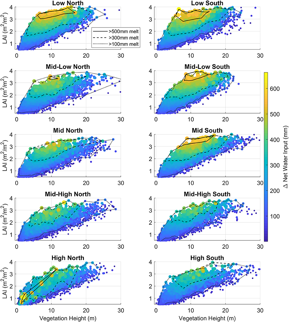
Figure 6. Forest patch (30 m) increase in total net water input across Snow Zones for both thinning scenarios and organized by existing vegetation LAI and height. Dots are colored and sized according to changes to net water input. Continuous, dashed and pointed lines show the boundary of points with changes in melt volume >500, 300, and 100 mm, respectively.

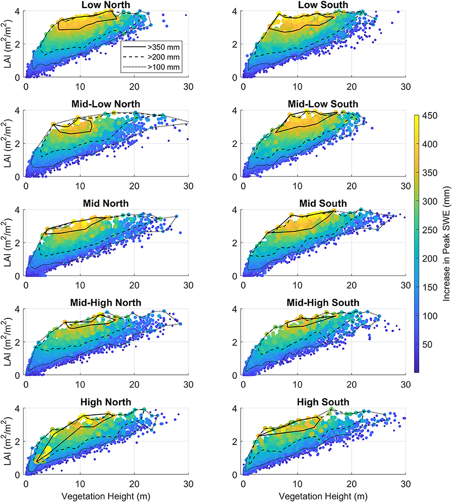
Figure 7. Forest patch (30 m) increase in peak SWE across Snow Zones for both thinning scenarios and organized by existing vegetation LAI and height. Dots are colored and sized according to increases in peak SWE. Continuous, dashed and pointed lines show the boundary of points with changes in melt volume >350, 200, and 100 mm, respectively.

Changes to peak SWE (Figure 7) show similar patterns to net water input (Figure 6 and Supplementary Figure 12), with relatively dense (LAI >3 m²/m²) and between 5 and 15 m tall pre-existing forest patches showing the largest SWE increases (>350 mm). However, unlike changes in net water input, some relatively dense (LAI > 3 m²/m²) forest patches with large peak SWE changes are also found at high elevations. Both positive and negative changes to mean daily incoming net radiation during snow covered days can be found across Snow Zones (Supplementary Figures 4, 5), due to the spatially uneven increase in solar radiation and decrease in longwave radiation produced by thinning. Forest patches that experience the largest decrease in incoming net radiation are those with low initial LAI (<2 m²/m²) and relatively short heights (<5 m) (Supplementary Figure 5). These areas are already significantly exposed to solar radiation and, therefore, the decrease in longwave radiation from removing warm trees outweighs the relatively smaller increase in shortwave radiation.

Changes to Mass and Energy Fluxes

Figure 8 shows changes of mass and energy fluxes, normalized by changes in LAI (Supplementary Table 1) for both thinning scenarios and the control run. Results from the 10 and 20-m thinning scenarios are aggregated to create an average normalized response to thinning. Changes to canopy sublimation drive the majority of changes to peak SWE and snowmelt. Snowmelt is separated from rain falling through snowpack in this analysis to adequately account for changes to the mass balance due to forest thinning. On average, melt volume changes are about 100 mm/m²m⁻² for all Snow Zones, when averaging data for all water years and for both thinning scenarios. However, there are differences in melt volume changes across years, where the wet and normal (WY17 and WY16, respectively) years are more sensitivity to LAI changes (uniformly 100–150 mm/m²m⁻² across all snow zones), and the dry year (WY18) shows smaller sensitivity to LAI changes and more variability among Snow Zones. In WY18, increasing melt volume and peak SWE were smaller at lower elevations with more rain-on-snow occurring at lower elevations. This is explained by the fact that the snow season was lengthened on average by about a week at lower elevations following tree removal, which allowed later rainfall events to be added to the remaining snowpack. Overall, normalized changes to snowmelt range from about 50 mm/m²m⁻² for the dry year (WY18) up to about 150 mm/m²m⁻² for the wet year (WY17) at mid to low elevations. Normalized changes to snowpack sublimation (both increasing and decreasing) are relatively small, due to the compensating effects between increasing incoming shortwave radiation and decreasing incoming longwave radiation following tree removal (lower panels Figure 8).

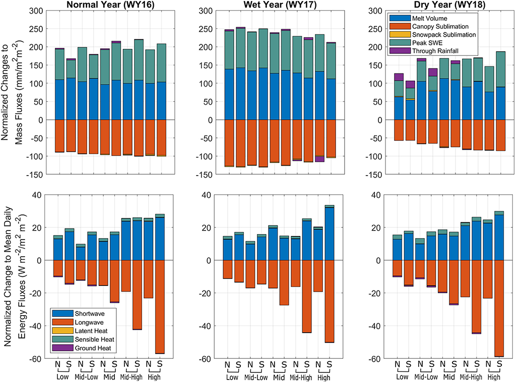
Figure 8. Upper panels: changes to the mean total mass fluxes normalized by LAI changes between the thinning scenarios and the control run. Lower panels: changes to the mean daily energy fluxes normalized by LAI changes. Values from both thinning scenarios are used.

Relatively little inter annual variability was found across Snow Zones for the energy flux changes (lower panel Figure 8). The largest changes to the energy fluxes are from increasing incoming shortwave radiation and decreasing incoming longwave radiation. Normalized changes to incoming shortwave radiation increase with elevation, opposite to the decrease of incoming longwave radiation with elevation. The net result of these compensating factors is that average changes to incoming net radiation are relatively small. The relationship between changes to incoming radiation with elevation is a result of the correlation between elevation, forest cover and slope, where higher elevations have sparser forest and steeper slopes (Figure 2). Steeper slopes mean that at times of low solar angles (winter and early melt season), more incoming solar radiation is available on south-facing slopes; therefore, after thinning, relatively more incoming solar radiation reaches the snowpack on higher-elevation south-facing slopes. Moreover, in sparser forests (typically found at high elevations), there are relatively fewer trees remaining after thinning to provide shelter from the sun. The opposite is true of denser forests, such as those found at lower elevations. Incoming longwave radiation shows the opposite pattern, where high elevation and south-facing Snow Zones have the largest decrease due to removal of warm trees emitting longwave.

Figure 9 presents time series of cumulative mass flux and SWE changes between the 20-m thinning scenario and the control run. This scenario is selected to analyze the largest expected changes to the timing of mass flux changes. Net water input shows that more early- and mid-winter events occur at lower elevations, producing earlier snowmelt than in the control run. Changes to SWE show that for the higher Snow Zones, there is a larger negative change (i.e., control run has higher SWE) before it reaches zero, suggesting a faster melting rate and an average earlier date of snow depletion after thinning (Figure 10). On average, at the High North-Facing Snow Zone, snow does not disappear during the wet WY17 (Figure 9), as SWE changes stay below zero (more snow in the control run) until end of WY17, due to significant snowfall that year. Changes to snowpack sublimation are minimal (< ±3 mm), particularly when compared to changes to the other mass fluxes. Changes in the number of snow-covered days and the date of snow disappearance after thinning are inconsistent across water years (Figure 10). However, the wet WY17 nearly always has a decrease in both snow-covered days and earlier date of snow disappearance following thinning, up to about 8 and 4.5 days, respectively (for the Mid to High North-Facing Snow Zones). The other water years showed a more variable response that generally reflects more snow-covered days and later snow disappearance following tree removal at lower elevation that shifts to less snow-covered days at higher elevations and north-facing Snow Zones (Figure 10).

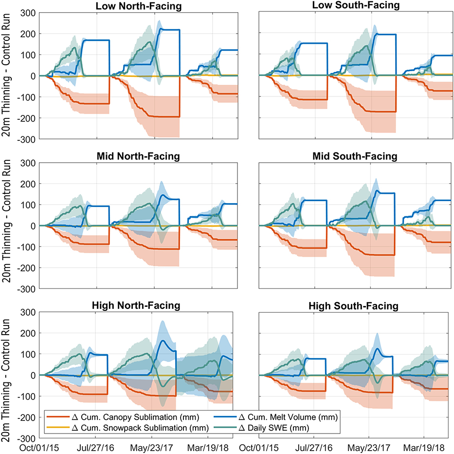
Figure 9. Time series of changes to cumulative mass fluxes and daily SWE for six representative Snow Zones between the 20-m thinning scenario and the control run.

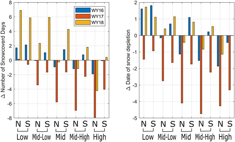
Figure 10. Mean changes in the number of snow-covered days and the date of snow depletion across Snow Zones between the two thinning scenarios and the control run.

Decision Support Tool: Random Forest (RF) Model

SnowPALM results are used to train the RF models to synthetize results and expand the analysis to neighboring watersheds. The out-of-bag RMSE and correlation coefficient of the RF models for each Snow Zone show overall good model performance (left panel Figure 11). RMSEs are similar to those found for the linear relationship between changes of LAI and total melt volume (Figure 5), and the correlation coefficients are consistently high (r² > 0.8). Out-of-bag mean bias was also calculated and it was below 0.1% for all the models, suggesting that the RF models are skillful and can be used to predict changes to net water input. The RF analysis shows that, not surprisingly, LAI change is the key driving variable for predicting changes to net water input across Snow Zones, followed by the LAI and height of existing vegetation (right panel Figure 11). Topographic variables have relatively little impact on the model; however, Snow Zones are already classified by topographic variability, reducing the relative importance of these variables. We also trained a Random Forest model using all the data, without classifying by Snow Zones, and that analysis shows a similar pattern, as variables associated with vegetation structure explain more than 90% of the changes to snowmelt volume.

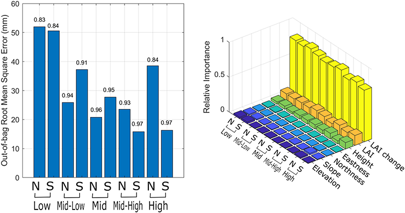
Figure 11. Left panel: out-of-bag root mean square error (y-axis) and correlation (numbers on top of bars) for the Random Forest models at each Snow Zone. Right panel: relative importance factors of the predictor variables used in the Random Forest model.

Figure 12 shows the simulated impacts of two forest thinning scenarios (0.6 and 2.4 mm²/mm² removal) using the trained RF model on the net water input of relatively dense (LAI = 3 m²/m²) and 10-m tall forest patches across different topographic conditions. We show these two scenarios as they represent a moderate and a severe thinning, which can be qualitatively associated with the 10 and 20-m thinning scenarios implemented in SnowPALM. The severe forest removal scenario increases melt volume three times more than the moderate scenario, with a maximum change of 310 mm for south-facing (northness >0) and mid-elevation (~2,200 masl) slopes. In both scenarios, thinning above ~2,300 masl produces lower melt volume increases than lower elevations. Similarly, thinning of low elevation (<2,100 m) areas also produce lower melt volume increases, particularly for the severe forest thinning scenario, compared to those between 2,100 and 2,300 m. Changes in elevation were associated with larger differences than changes in aspect (Figure 12); however, south-facing slopes generally benefitted more from thinning, especially at elevations <2,200 m. These results generally agree with those presented in the previous section, where thinning mid-elevation and south-facing Snow Zones produce the largest changes to net water input (Figure 5).

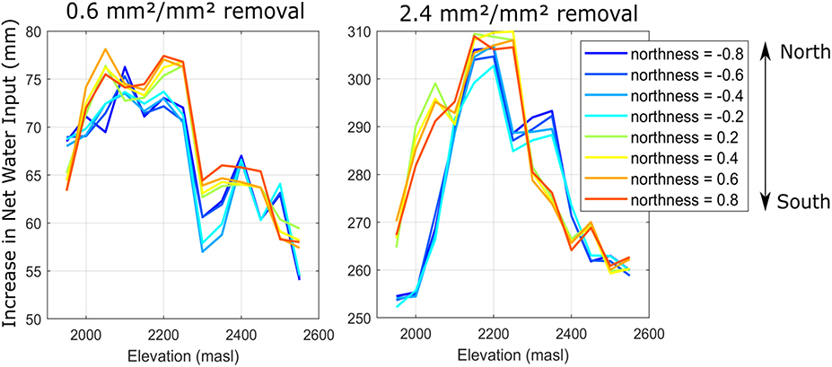
Figure 12. Predicted increase in the total melt volume by the Random Forest model for a dense forest patch with mean LAI and height of 3 m²/m² and 10 m, respectively, and two thinning scenarios: moderate (0.6 m²/m²) and significant (2.4 m²/m²) thinning. A negative northness index represents a more north oriented slope, with−1 representing a completely north-facing slope.

We applied the RF model to 12 watersheds across the west shore of Lake Tahoe (Supplementary Figure 8), as an example of an application of the decision support tool. These watersheds span from Burton Creek in the North to Cascade Creek to the South of Lake Tahoe. Drainage area varies from about 29 km² for Blackwood Creek to about 1.7 km² for the Little Rubicon Creek. These watersheds have different degrees of vegetation cover and topographic gradients. The RF model was applied only to forest patches with LAI >3 m²/m² and height between 5 and 15 m, which are the most sensitive to forest removal (Figure 7). Five thinning scenarios of 0.7, 1.4, 2.1, 2.8, and 3.5 m²/m² LAI removal in each 30-m forest patch scale were investigated, representing scenarios of minimal to severe intervention. The watersheds with the largest number of targeted forest patches per km² are Burton Creek and Little Rubicon at about 120 km⁻². The average impact on melt volume is 80–380 mm for the 0.7 and 3.5 m²/m² LAI removal, respectively (center panel Figure 13). The normalized change in melt volume suggests that there is not much variability in the sensitivity of these watersheds to forest thinning. The Little Rubicon Creek Watershed is the most sensitive (120 mm/m²m²) to forest removal and Eagle Creek watershed the least sensitive (107 mm/m²m²) to changes in melt volume, a difference of only 11%. These minor differences across watersheds are consistent with their similar topography and the dominant role of vegetation structure.

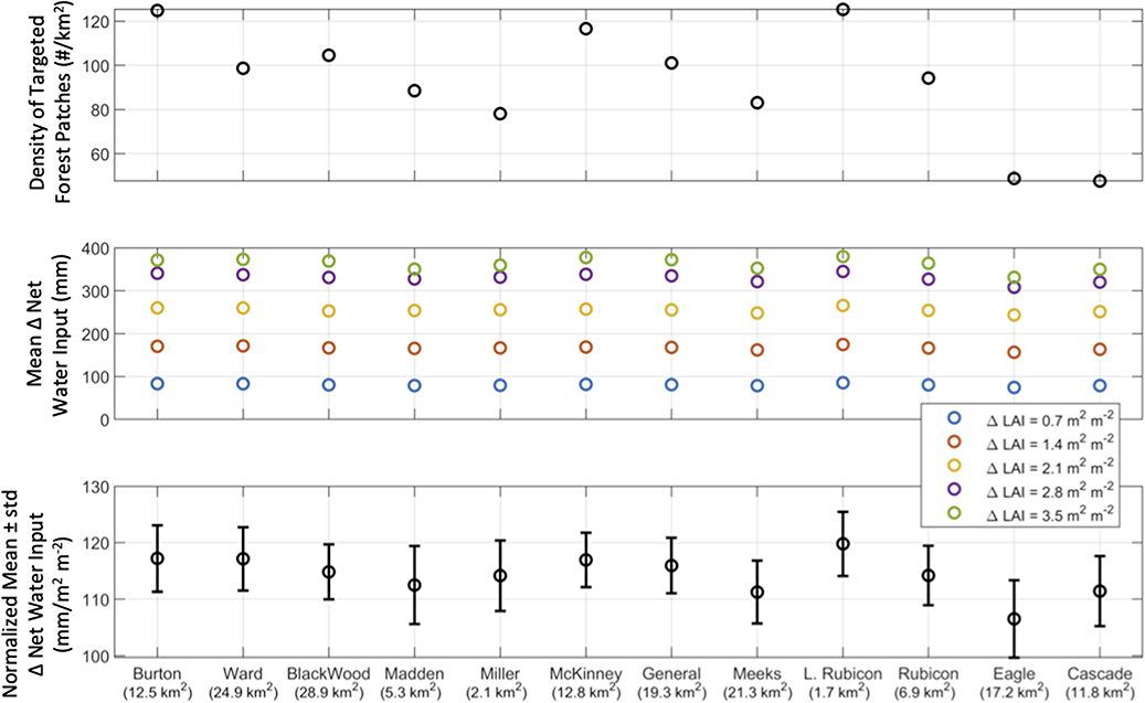
Figure 13. Upper panel: density of targeted forest patches (LAI > 3 m²/m² and height between 5 and 15 m) across 12 watersheds on the west shore of Lake Tahoe. Center panel: expected change to net water input for the targeted forest patches and each thinning scenario. Lower panel: mean and standard deviation of the expected normalized changes to net water input. Watersheds in the X-axis are sorted from north to south (left to right) and the drainage area is also presented for comparison.

Discussion

In this study, we use high resolution (1 m) and large-extent (>50 km²) spatially explicit snow modeling to predict the impact that landscape-scale forest thinning will have on snowpack along the west shore of Lake Tahoe. We find that in general, forest thinning decreases canopy sublimation, resulting in greater peak SWE and melt volumes (Figure 8). Because of this, the 20-m thinning scenario (most aggressive) produced the largest increases in snow accumulation and melt. Changes in incoming net radiation are relatively small due to compensating effects of decreasing incoming longwave radiation and increasing incoming shortwave radiation that accompany the forest cover changes (Supplementary Figure 9). This results in relatively small changes to snowpack sublimation, which only reach values up to about 25 mm (Supplementary Figure 6). Despite broad increases in melt volumes following tree removal, the snowpack response of any given 30-m forest patch depends on topographic position, existing vegetation structure and the seasonal climate variability. Our implications are consistent with those from Harpold et al. (2020), suggesting that relatively dense and shorter forest patches produce the largest increase in melt volume. However, the significantly larger domain and more variable climatic conditions used in the study, allowed insight into the transferability across topographic conditions (e.g., aspect and elevation) and identified watersheds where melt volumes would benefit most from thinning.

Our results help to place previous field observations of forest cover effects on snow accumulation and ablation into context. The model results show that decreasing forest cover tends to increase snow accumulation and increase ablation rates, in general agreement with a meta-analysis of 33 studies (Varhola et al., 2010) (Figure 14). In particular, our results agree with those from the nearby Central Sierra Snow Laboratory in the 1950's (Anderson and Gleason, 1960; Anderson et al., 1976) (green dots, Figure 14), in which their variability falls within the inter-patch variability found in our study (blue dashed lines, Figure 14). The sensitivity of snow ablation (melt volume + snowpack sublimation) to changes in forest cover in Lake Tahoe are somewhat smaller than the Varhola et al. (2010) dataset. Future pre- and post-thinning observations will be challenged to account for inter-annual climate variability and the effects of topography, which may cause substantial variability in stand-scale analyses (e.g., Varhola et al., 2010) limiting out ability to provide generalized inferences and recommendations across regions.

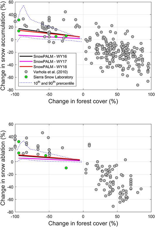
Figure 14. Changes in peak snow accumulation (upper) and snow ablation (melt + snowpack sublimation) (lower) against changes in forest cover comparing the data from Varhola et al. (2010, Figure 8) meta-analysis and linear regressions for the three water years and both thinning scenarios simulated by SnowPALM at a 30-m forest stand scale. Dashed lines show the 10th and 90th percentile of all the 30-m forest stands used in the regression lines. Green dots highlight those points from Varhola et al. (2010) that are the closest to our study domain.

We find that differences due to forest thinning are highly dependent on the spatial distribution of trees. For example, the largest changes to canopy sublimation and snow accumulation are found in stands that are dense (LAI > 3 m²/m²) and between 5 and 15-m tall (Figures 6, 7). These most responsive forest stands can increase peak SWE by about 400–450 mm (Figure 7) or more than 60% in the 20-m thinning scenario. Spatial patterns of increases and decreases of snowpack sublimation are also highly dependent on forest geometry and its change (Supplementary Figure 6). Relatively open areas exhibit decreasing snowpack sublimation, while areas around tree clusters increase snowpack sublimation (Figure 4). However, limitations associated with the representation of wind fields and turbulent fluxes remain one of the key uncertainties in modeling forest environments, where current approaches can lead to compensating modeling errors (Conway et al., 2018). Forest thinning also increases and decreases net incoming radiation, due to tradeoffs between increasing incoming shortwave and decreasing incoming longwave radiation by removing warm trees that shade nearby snowpack. Open areas on the south edges of trees removed by thinning show a decrease in net incoming radiation leading to relatively small snowpack changes (Figure 4). Conversely, areas with denser forest cover have an increase in net incoming radiation; however, changes to snowpack in these places are mostly controlled by changes in canopy sublimation.

Pre- and post-thinning forest structure and climate are the primary controls on snow accumulation and melt, with large-scale topography having a secondary effect that is likely related to the co-dependence between forests structure and topography. For example, we find that lower elevation Snow Zones have the largest absolute snowpack changes (Supplementary Figure 6), and the lowest snowfall, because low elevation forests are generally denser (Figure 2). The impact of forest thinning on the high north-facing Snow Zone is somewhat distinct, as thinning enhances wind speed and increases snow redistribution by wind, which produces areas of preferential snow accumulation that are not found in other Snow Zones (Figure 7). Inter-annual climate variability is a more important control than topography in terms of the relative impact of thinning on the snowpack. For example, relative changes to net water input for the 20-m thinning scenario are larger during dry years (16% of the control run) than wet years (7% of the control run) (Supplementary Figure 10). This suggests that positive effects of thinning on net water input are greatest when water is needed the most (dry years), representing an important and positive co-benefit for forest health and water supply.

We use these model results to train a novel decision support tool to predict the greatest potential to increase water yields and identify co-benefits to other resources from forest thinning. The goal of the tool is to provide guidance to resource managers on how to incorporate hydrologic interests, such as increasing water yield, snow melt volumes and snow duration, into landscape restoration strategies that seek to achieve multiple benefits. In general, retaining snow longer on the landscape delays the timing of water inputs, which leads to a shorter period of soil water stress (Harpold, 2016) and reduces severe fire risk (Westerling et al., 2006). Historically in the Sierra Nevada, montane conifer forests were dominated by tall, large diameter trees that were variably distributed across the landscape (North et al., 2009). Fire suppression and timber harvest over the past 100 years has resulted in much higher densities of smaller diameter trees occurring consistently across large areas, particularly at low to moderate elevations. Forest restoration efforts intended to promote habitat in Sierra Nevada forests are designed to decrease the density of shorter, smaller diameter trees, increase the occurrence of larger trees, and increase the heterogeneity of their spatial distribution across the landscape toward an array of tree clumps and gaps (North et al., 2009). These ideal forest characteristics are more closely matched to our synthetically thinned forest than the existing forest (Figure 4). High density stands are more likely to carry high intensity fire (Collins et al., 2011), and topography can have a substantial effect on fire intensity as well (e.g., Harris and Taylor, 2015). South-facing slopes are less likely to carry high intensity fire because they tend to have lower tree densities compared to north-facing slopes, but they also experience greater solar radiation, so high tree densities are more likely to experience drought stress (Underwood et al., 2010). Therefore, targeting high density forest patches in south-facing slopes is a high priority that is further supported by this study (Figures 6, 12). North-facing slopes, alternatively, are typically cooler and can be more suitable for supporting forests with higher canopy density and associated forest plants and wildlife. Thus, forest restoration, fire risk management, and wildlife habitat conservation can be reconciled with forest thinning effects on net water input, and in fact can have positive feedbacks that promote co-benefits for water availability during dry periods (Boisramé et al., 2018).

Summary and Conclusion

Changes to LAI in 30-m forest patches with specific pre-existing vegetation structure (LAI > 3 m²/m² and between 5 and 15-m tall) produce the largest increase in snow accumulation and melt volume. Macro-topography has a secondary role in predicting changes to snowpack following tree removal. Mid to low elevation (<2,300 masl) and south-facing areas were found to produce the largest increase in snow accumulation and melt after thinning. Forest thinning strategies in those forest patches are informed by a decision-support tool that recommends slightly different tree removal strategies in different topographic positions. We found that these recommendations are generally consistent with co-management for multiple resource goals, such as fire suppression, wildlife habitat conservation and water conservation, which is a key to maximizing resources invested into expanding forest restoration efforts.

In this study, we take an early step to develop a computationally efficient tool that is easy to implement for forest managers to predict changes to snowpack after thinning that resolves tree-scale processes. Given the lack of high-resolution models like SnowPALM, our simulations and the decision support tool derived from them are a novel means to translate information to nearby watersheds and different conditions. Challenges remain, however, in refining and verifying models like SnowPALM and implementing them in domains large enough to resolve primary snow forest controls across a range of vegetation and climate conditions. For example, the east shore of Lake Tahoe has a much different climate and dominant tree species that may not coincide with the recommendations made here. Another area where current forest planning is lacking is understanding the long-term impact of forest thinning on the water budgets. Processes such as compensating tree water use, under story, and tree regrowth may impact the long term efficiency of thinning. The scale of forest restoration needed for fuel management is significant in the Sierra Nevada (Kirwan et al., 2014), and represents one of the few ways that humans can manage their upland water supply systems. Given this societal need, continued work at the interface of basic process research and large-scale forest restoration applications are an avenue that could yield important advances.

Data Availability Statement

The datasets generated for this study are available on request to the corresponding author.

Author Contributions

SK, AH, and PB designed the study. SK and PB conducted snow simulation with SnowPALM. SK analyzed SnowPALM outputs with help from AH and PB. SK, AH, PB, and PM contributed to writing and overall discussion of results.

Funding

Financial support for this study was provided by the USFS via the Tahoe West Project and the State of California Wildlife Conservation Board.

Conflict of Interest

The authors declare that the research was conducted in the absence of any commercial or financial relationships that could be construed as a potential conflict of interest.

Acknowledgments

Authors thank A. Varhola for providing some of the data used in Figure 14. We thank Jonathan Greenberg for developing the tree segmentation data used. SnowPALM simulations were run at the Arizona Remote Sensing Center and at the University of Nevada, Reno, using computing resources from the Nevada Mountain Ecohydrology Lab. Comments from two reviewers are greatly appreciated.

Supplementary Material

The Supplementary Material for this article can be found online at: https://www.frontiersin.org/articles/10.3389/ffgc.2020.00021/full#supplementary-material

References

Alexander, R. R., Troendle, C. A. A., Kaufmann, M. R., Shepperd, W. D., Crouch, G. L., and Watkins, R. K. (1985). The fraser experimental forest colorado: research program and published research 1937-1985. Fort Collins: U.S. Dept. of agriculture, Forest Service, Rocky Mountain Forest and Range Experiment Station. Available online at: https://www.fs.fed.us/rm/pubs_rm/rm_gtr118.pdf (accessed March 03, 2020).
Anderson, H. W. (1956). Forest-cover effects on snowpack accumulation and melt, central sierra snow laboratory. Eos Trans. Am. Geophys. Union 37, 307–312. doi: 10.1029/TR037i003p00307
Anderson, H. W. (1963). Managing California's Snow Zone Lands For Water. Available online at: http://citeseerx.ist.psu.edu/viewdoc/download?doi=10.1.1.224.4871&rep=rep1&type=pdf (accessed March 03, 2020).
Anderson, H. W., and Gleason, C. H. (1960). Effects of logging and brush removal on snow water runoff. Int. Assoc. Hydrol. Sci. Publ. 51, 478–489.
Anderson, H. W., Hoover, M., and Reinhart, K. G. (1976). Forests and Water: Effects of Forest Management on Floods, Sedimentation, and Water Supply. Berkley, CA. Available online at: https://www.fs.usda.gov/treesearch/pubs/24048 (accessed March 03, 2020).
Bewley, D., Alila, Y., and Varhola, A. (2010). Variability of snow water equivalent and snow energetics across a large catchment subject to mountain pine beetle infestation and rapid salvage logging. J. Hydrol. 388, 464–479. doi: 10.1016/j.jhydrol.2010.05.031
Blöschl, G. (1999). Scaling issues in snow hydrology. Hydrol. Process. 13, 2149–2175. doi: 10.1002/(SICI)1099-1085(199910)13:14/15<2149::AID-HYP847>3.0.CO;2-8
Boisramé, G., Thompson, S., and Stephens, S. (2018). Hydrologic responses to restored wildfire regimes revealed by soil moisture-vegetation relationships. Adv. Water Resour. 112, 124–146. doi: 10.1016/j.advwatres.2017.12.009
Broxton, P. D., Harpold, A. A., Biederman, J. A., Troch, P. A., Molotch, N. P., and Brooks, P. D. (2015). Quantifying the effects of vegetation structure on snow accumulation and ablation in mixed-conifer forests. Ecohydrology 8, 1073–1094. doi: 10.1002/eco.1565
Church, J. E. (1933). Snow surveying: its principles and possibilities. Geogr. Rev. 23, 529–563. doi: 10.2307/209242
Collins, B. M., Everett, R. G., and Stephens, S. L. (2011). Impacts of fire exclusion and recent managed fire on forest structure in old growth Sierra Nevada mixed-conifer forests. Ecosphere 2, 1–4. doi: 10.1890/ES11-00026.1
Conway, J. P., Pomeroy, J. W., Helgason, W. D., and Kinar, N. J. (2018). Challenges in modeling turbulent heat fluxes to snowpacks in forest clearings. J. Hydrometeorol. 19, 1599–1616. doi: 10.1175/JHM-D-18-0050.1
Deardorff, J. W. (1978). Efficient prediction of ground surface temperature and moisture, with inclusion of a layer of vegetation. J. Geophys. Res. 83:1889–1903. doi: 10.1029/JC083iC04p01889
Essery, R., Rutter, N., Pomeroy, J., Baxter, R., Stähli, M., Gustafsson, D., et al. (2009). SNOWMIP2: An evaluation of forest snow process simulations. Bull. Am. Meteorol. Soc. 90, 1120–1136. doi: 10.1175/2009BAMS2629.1
Golding, D. L., and Swanson, R. H. (1986). Snow distribution patterns in clearings and adjacent forest. Water Resour. Res. 22, 1931–1940. doi: 10.1029/WR022i013p01931
Goodell, B. (1952). Watershed-management aspects of thinned young lodgepole pine stands. J. For. 50, 374–378. doi: 10.1093/jof/50.5.374
Harpold, A. A. (2016). Diverging sensitivity of soil water stress to changing snowmelt timing in the Western U.S. Adv. Water Resour. 92, 116–129. doi: 10.1016/j.advwatres.2016.03.017
Harpold, A. A., and Brooks, P. D. (2018). Humidity determines snowpack ablation under a warming climate. Proc. Natl. Acad. Sci.U. S. A. 115, 1215–1220. doi: 10.1073/pnas.1716789115
Harpold, A. A., Krogh, S. A., Kohler, M., Eckberg, D., Greenberg, J., Sterle, G. (2020). “Increasing the efficacy of forest thinning for snow using high-resolution modeling: a proof of concept in The Lake Tahoe Basin, California, USA” in Ecohydrology. doi: 10.1002/eco.2203
Harris, L., and Taylor, A. H. (2015). Topography, fuels, and fire exclusion drive fire severity of the rim fire in an old-growth mixed-conifer forest, yosemite national park, USA. Ecosystems 18, 1192–1208. doi: 10.1007/s10021-015-9890-9
Kirwan, B. J., Branham, J., and Keegan, J. (2014). The State of The Sierra Nevada's Forests. Available online at: https://sierranevada.ca.gov/wp-content/uploads/sites/236/attachments/StateOfSierraForestsRptWeb.pdf (accessed March 03, 2020).
López-Moreno, J. I., Pomeroy, J. W., Revuelto, J., and Vicente-Serrano, S. M. (2013). Response of snow processes to climate change: spatial variability in a small basin in the spanish pyrenees. Hydrol. Process. 27, 2637–2650. doi: 10.1002/hyp.9408
Mahat, V., and Tarboton, D. G. (2012). Canopy radiation transmission for an energy balance snowmelt model. Water Resour. Res. 48, 1–16. doi: 10.1029/2011WR010438
Moeser, D., Roubinek, J., Schleppi, P., Morsdorf, F., and Jonas, T. (2014). Canopy closure, LAI and radiation transfer from airborne LiDAR synthetic images. Agric. For. Meteorol. 197, 158–168. doi: 10.1016/j.agrformet.2014.06.008
Moeser, D., Stahli, M., Jonas, T., Stähli, M., Jonas, T., Stahli, M., et al. (2015). Improved snow interception modeling using canopy parameters derived from airborne LIDAR data. Water Resour. Res. 51, 5041–5059. doi: 10.1002/2014WR016724
Mote, P. W., Li, S., Lettenmaier, D. P., Xiao, M., and Engel, R. (2018). Dramatic declines in snowpack in the western US. npj Clim. Atmos. Sci. 1:2. doi: 10.1038/s41612-018-0012-1
Musselman, K. N., Clark, M. P., Liu, C., Ikeda, K., and Rasmussen, R. (2017a). Slower snowmelt in a warmer world. Nat. Clim. Chang. 7, 214–219. doi: 10.1038/nclimate3225
Musselman, K. N., Pomeroy, J. W., Centre, O., Musselman, K. N., and Pomeroy, J. W. (2017b). Estimation of needleleaf canopy and trunk temperatures and longwave contribution to melting snow. J. Hydrometeorol. 18, 555–572. doi: 10.1175/JHM-D-16-0111.1
Musselman, K. N., Pomeroy, J. W., and Link, T. E. (2015). Variability in shortwave irradiance caused by forest gaps: measurements, modelling, and implications for snow energetics. Agric. For. Meteorol. 207, 69–82. doi: 10.1016/j.agrformet.2015.03.014
North, M., Stine, P., O'Hara, K., Zielinski, W., and Stephens, S. (2009). An Ecosystem Management Strategy For Sierran Mixed- Conifer Forests. Available online at: https://www.fs.fed.us/psw/publications/documents/psw_gtr220/psw_gtr220.pdf (accessed March 03, 2020).
Petersky, R. S., Shoemaker, K. T., Weisberg, P. J., and Harpold, A. A. (2018). The sensitivity of snow ephemerality to warming climate across an arid to montane vegetation gradient. Ecohydrology 12, 1–14. doi: 10.1002/eco.2060
Pomeroy, J. W., and Granger, R. J. (1997). “Sustainability of the western canadian boreal forest under changing hydrological conditions. I. snow accumulation and ablation,” in Sustainability of Water Resources under Increasing Uncertainty, eds. D. Rosjberg, N. Boutayeb, A. Gustard, Z. Kundzewicz, and P. Rasmussen (Wallingford: International Association of Hydrological Sciences) (IAHS Publ. No. 240), 237–242.
Pomeroy, J. W., Gray, D. M., Hedstrom, N. R., and Janowicz, J. R. (2002). Prediction of seasonal snow accumulation in cold climate forests. Hydrol. Process. 16, 3543–3558. doi: 10.1002/hyp.1228
Pomeroy, J. W., Parviainen, J., Hedstrom, N., and Gray, D. M. (1998). Coupled modelling of forest snow interception and sublimation. Hydrol. Process. 12, 2317–2337. doi: 10.1002/(SICI)1099-1085(199812)12:15<2317::AID-HYP799>3.0.CO;2-X
Rutter, N., Essery, R., Pomeroy, J., Altimir, N., Andreadis, K., Baker, I., et al. (2009). Evaluation of forest snow processes models (SnowMIP2). J. Geophys. Res. 114:D06111. doi: 10.1029/2008JD011063
Sturm, M., Goldstein, M. A., and Parr, C. (2017). Water and life from snow: a trillion dollar science question. Water Resour. Res. 53, 3534–3544. doi: 10.1002/2017WR020840
Tague, C. L., Moritz, M., and Hanan, E. (2019). The changing water cycle: the eco-hydrologic impacts of forest density reduction in Mediterranean (seasonally dry) regions. Wiley Interdiscip. Rev. Water 6:e1350. doi: 10.1002/wat2.1350
Tinkham, W. T., Smith, A. M. S., Marshall, H. P., Link, T. E., Falkowski, M. J., and Winstral, A. H. (2014). Quantifying spatial distribution of snow depth errors from LiDAR using random forest. Remote Sens. Environ. 141, 105–115. doi: 10.1016/j.rse.2013.10.021
Toews, D. A. A., and Gluns, D. R. D. R. (1986). “Snow accumulation and ablation on adjacent forested and clearcut sites in southeastern British Columbia,” in 54th Western Snow Conference (Phoenix, AZ), 12.
Troendle, C. A., and Leaf, C. F. (1980). “Hydrology,” in An Apporach to Water Resources Evaluation of Non-Point Silvicultural Sources: (A Procedural Handbook), Washington, DC: U.S. Environmental Protection Agency.
Underwood, E. C., Viers, J. H., Quinn, J. F., and North, M. (2010). Using topography to meet wildlife and fuels treatment objectives in fire-suppressed landscapes. Environ. Manage. 46, 809–819. doi: 10.1007/s00267-010-9556-5
van Gunst, K. J. (2012). Forest mortality in Lake Tahoe Basin from 1985-2010: influences of forest type, stand density, topography and climate (Master's degree thesis). Department of Natural Resources and Environmental Science, University of Nevada, Reno, NV, USA. Available online at: https://scholarworks.unr.edu/handle/11714/3773 (accessed March 03, 2020).
Varhola, A., Coops, N. C., Weiler, M., and Moore, R. D. (2010). Forest canopy effects on snow accumulation and ablation: an integrative review of empirical results. J. Hydrol. 392, 219–233. doi: 10.1016/j.jhydrol.2010.08.009
Westerling, A. L., Hidalgo, H. G., Cayan, D. R., and Swetnam, T. W. (2006). Warming and earlier spring increase western U.S. forest wildfire activity. Science 313, 940–943. doi: 10.1126/science.1128834
Winkler, R. D., Spittlehouse, D. L., and Golding, D. L. (2005). Measured differences in snow accumulation and melt among clearcut, juvenile, and mature forests in southern British Columbia. Hydrol. Process. 19, 51–62. doi: 10.1002/hyp.5757
Winstral, A., and Marks, D. (2002). Simulating wind fields and snow redistribution using terrain-based parameters to model snow accumulation and melt over a semi-arid mountain catchment. Hydrol. Process. 16, 3585–3603. doi: 10.1002/hyp.1238
Woods, S. W., Ahl, R., Sappington, J., and McCaughey, W. (2006). Snow accumulation in thinned lodgepole pine stands, Montana, USA. For. Ecol. Manage. 235, 202–211. doi: 10.1016/j.foreco.2006.08.013
Xia, Y., Mitchell, K., Ek, M., Sheffield, J., Cosgrove, B., Wood, E., et al. (2012). Continental-scale water and energy flux analysis and validation for the North American land data assimilation system project phase 2 (NLDAS-2): 1. Intercomparison and application of model products. J. Geophys. Res. Atmos. 117, 1–27. doi: 10.1029/2011JD016051
Keywords: snow hydrology, modeling, lidar, forest, forest management, restoration
Citation: Krogh SA, Broxton PD, Manley PN and Harpold AA (2020) Using Process Based Snow Modeling and Lidar to Predict the Effects of Forest Thinning on the Northern Sierra Nevada Snowpack. Front. For. Glob. Change 3:21. doi: 10.3389/ffgc.2020.00021
Received: 27 November 2019; Accepted: 24 February 2020;
Published: 20 March 2020.
Edited by:
Steven George Mcnulty, USDA Southeast Climate Hubs, United StatesReviewed by:
John L. Campbell, Northern Research Station, Forest Service (USDA), United StatesFengjing Liu, Michigan Technological University, United States
Copyright © 2020 Krogh, Broxton, Manley and Harpold. This is an open-access article distributed under the terms of the Creative Commons Attribution License (CC BY). The use, distribution or reproduction in other forums is permitted, provided the original author(s) and the copyright owner(s) are credited and that the original publication in this journal is cited, in accordance with accepted academic practice. No use, distribution or reproduction is permitted which does not comply with these terms.
*Correspondence: Sebastian A. Krogh, skrogh@cabnr.unr.edu; sebakrogh@gmail.com