


Abstract
We present a radial velocity (RV) analysis of TOI-1136, a bright Transiting Exoplanet Survey Satellite (TESS) system with six confirmed transiting planets, and a seventh single-transiting planet candidate. All planets in the system are amenable to transmission spectroscopy, making TOI-1136 one of the best targets for intra-system comparison of exoplanet atmospheres. TOI-1136 is young (∼700 Myr), and the system exhibits transit timing variations (TTVs). The youth of the system contributes to high stellar variability on the order of 50 m s−1, much larger than the likely RV amplitude of any of the transiting exoplanets. Utilizing 359 High Resolution Echelle Spectrometer and Automated Planet Finder RVs collected as part of the TESS-Keck Survey, and 51 High-Accuracy Radial velocity Planetary Searcher North RVs, we experiment with a joint TTV-RV fit. With seven possible transiting planets, TTVs, more than 400 RVs, and a stellar activity model, we posit that we may be presenting the most complex mass recovery of an exoplanet system in the literature to date. By combining TTVs and RVs, we minimized Gaussian process overfitting and retrieved new masses for this system: (mb−g = ,
,  ,
,  ,
,  ,
,  ,
,  M⊕). We are unable to significantly detect the mass of the seventh planet candidate in the RVs, but we are able to loosely constrain a possible orbital period near 80 days. Future TESS observations might confirm the existence of a seventh planet in the system, better constrain the masses and orbital properties of the known exoplanets, and generally shine light on this scientifically interesting system.
Export citation and abstract BibTeX RIS

Original content from this work may be used under the terms of the Creative Commons Attribution 4.0 licence. Any further distribution of this work must maintain attribution to the author(s) and the title of the work, journal citation and DOI.
1. Introduction
Among the most pressing scientific questions in the field of exoplanet science are those of planet formation and the subsequent evolution of planetary systems. Population studies are generally required to learn about such processes, as the involved astronomical timescales are far too long for direct observations. Multiple different processes might explain the formation of exoplanets in other systems: pebble accretion could form planets in situ (Lambrechts & Johansen 2012; Izidoro et al. 2021), or planets might form beyond the ice line and migrate inward (Goldreich & Tremaine 1980; D'Angelo et al. 2003; Raymond et al. 2008; Izidoro et al. 2017). The subsequent evolution of planets post formation, such as atmospheric sculpting from stellar flux (Lammer et al. 2003) or the outgassing of volatiles (Rogers et al. 2011), likely also affects the observed planetary population.
Challenges comparing different exoplanetary systems are compounded by the various natures of host stars: While it is possible to control for aspects such as age, stellar type, and metallicity when studying formation history, the probable dependence of system evolution on a variety of the host star's parameters makes wider study difficult. Consequently, multiple-planet systems are very attractive when studying planetary characteristics such as atmospheric evolution, as they all share a host star, allowing for the removal of degeneracies between different stellar parameters. Higher multiplicities are better, as they allow for a larger sample size that shares system parameters.
The successful launch of JWST (Gardner et al. 2006) places a particular emphasis on systems that are highly amenable to atmospheric characterization via transmission spectroscopy, as this is one of JWST's primary science goals. Early programs with JWST are already observing previously undetected exoplanet atmospheric features (JWST Transiting Exoplanet Community Early Release Science Team et al. 2023) and ruling out atmospheres in popular targets such as TRAPPIST-1 b (Greene et al. 2023).
Here we present a follow-up analysis of TOI-1136, a system with at least six transiting planets first characterized by Dai et al. (2023, hereafter D23), and a candidate seventh. TOI-1136 is a young (700 ± 100 Myr), bright (V = 9.5) G dwarf that has several planets that exhibit significant transit timing variations (TTVs), allowing for the precise characterization of most planet masses with photometry alone. The planets are in deep Laplace resonance (Pb = 4.1727 days, Pc = 6.2574 days, Pd = 12.5199 days, Pe = 18.801 days, Pf = 26.321 days, Pg = 39.545 days), suggesting a distinct formation history (short-scale Type I migration; Sinclair 1975; D23). TOI-1136 was observed by the Transiting Exoplanet Survey Satellite (TESS; Ricker et al. 2015) for six nonconsecutive sectors. The relatively short baseline of TESS limits the precision with which we can constrain planetary masses using TTVs, especially for the longer-period outer planets. Furthermore, adding radial velocities (RVs) in conjunction with TTVs can help prevent conflict between TTV-only and RV-only measured masses (Steffen 2016; Mills & Mazeh 2017).
The TESS-Keck Survey (TKS; Chontos et al. 2022) carried out extensive RV observations of TOI-1136 as part of its primary survey to measure the masses of 100 transiting planets. TKS is divided into a variety of science cases studying the radius gap first identified in Fulton et al. (2017; see also Weiss et al. 2021; Brinkman et al. 2023), orbital dynamics (MacDougall et al. 2021; Rubenzahl et al. 2021), multi-planet systems (Lubin et al. 2022; Turtelboom et al. 2022), and atmospheres (Scarsdale et al. 2021; Akana Murphy et al. 2023), to name a few. TOI-1136 fits almost every science case in TKS, and is consequently a very important system for the TKS team to understand.
We utilize over 400 RVs taken with the High Resolution Echelle Spectrometer (HIRES; Vogt et al. 1994), the Levy Spectrometer on the robotic Automated Planet Finder (APF; Vogt et al. 2014) Telescope, and the High-Accuracy Radial velocity Planetary Searcher North (HARPS-N; Cosentino et al. 2012) spectrograph. We combine these observations with TTVs and perform a detailed RV+TTV analysis of TOI-1136.
The paper is organized as follows. A summary of our observations and data is given in Section 2. A brief description of the stellar parameters of TOI-1136 is given in Section 3. A study of the candidate seventh planet is given in Section 4. Our analysis is detailed in Section 5. Finally, the results and their interpretation are placed into context in Section 6, and the paper is summarized in Section 7.
2. Observations
2.1. TESS Photometry
TOI-1136 was first observed by TESS during Sector 14 (2019 July 18–August 15) and Sector 15 (2019 August 15–September 11) of Cycle 2. TOI-1136 was later reobserved during Sectors 21 and 22 (2020 January 21–March 18), and in two subsequent sectors: Sectors 41 (2021 July 23–August 20) and 48 (2022 January 28–February 26). The star was first declared a TESS Object of Interest (TOI; Guerrero et al. 2021) on 2019 August 27, and the Science Processing and Operations Center (Jenkins et al. 2016) pipeline would eventually identify four candidate planets in the system. Additional community observers would later identify two more community TOIs (or CTOIs), increasing the number of candidate planets in the system to six.
No additonal TESS photometry has been acquired since the system was studied in D23. Nonetheless, the TESS photometry is incorporated in multiple aspects of our analysis of the system. We build on the individual transit times of the TOI-1136 planets determined in D23 by jointly modeling these transit times with RVs in Section 5. We also analyze the TESS Presearch Data Cleaning Simple Aperture Flux (PDCSAP; Jenkins et al. 2016) photometry to measure the stellar rotation period, to fit a single transit to the candidate planet in Section 4.1, and to calculate FF' values utilized in Section 5.1 by multiplying the PDCSAP flux (F) by its first derivative (F Aigrain et al. 2012).
2.2. Radial Velocities with Keck/HIRES
Between 2019 November 1 and 2022 July 16, we obtained 155 high-resolution spectra of TOI-1136, resulting in 103 nightly binned RV observations, using HIRES (Vogt et al. 1994), located at Keck Observatory. Precise RVs were extracted using a warm iodine cell in the light path for wavelength calibration, as described in Butler et al. (1996). We extracted precise RVs from the echelle spectra using the California Planet Search pipeline (Howard et al. 2010).
We typically achieved a signal-to-noise ratio (S/N) of ≈200 at visible wavlengths for each spectrum by capping the HIRES built-in exposure meter at 250,000 counts, resulting in a median nightly binned RV uncertainty of 1.75 m s−1 and a median S/N of 214 for the wavelength order centered at 540 nm.
2.3. HARPS-N Radial Velocities
We also utilized 51 RV observations of TOI-1136 obtained using the HARPS-N spectrograph at the Telescopio Nazionale Galileo, a 3.6 m telescope located in the Canary Islands, Spain under the observing programs CAT19A_162, ITP19_1, and CAT21A_119. Observations had a median exposure time of 1000 s and a median S/N of 74.6 at 550 nm.
HARPS-N RVs were reduced using the standard cross-correlation function mask method outlined in Baranne et al. (1996) and Pepe et al. (2002). After reduction, HARPS-N RVs had a mean uncertainty of 2.63 m s−1.
2.4. Radial Velocities with the Automated Planet Finder
Essential to characterizing the stellar activity were additional RV observations taken using the APF Telescope, located at Lick Observatory on Mount Hamilton, CA. The automated nature of the APF allowed for much more consistent, high-cadence observations than were possible using HIRES or HARPS-N. The smaller aperture of APF, however, restricted us to lower S/N and correspondingly less precise observations. Between 2019 November 1 and 2022 July 16, we carried out 320 APF observations over the course of 256 observing nights. APF spectra are calibrated using an iodine cell and are extracted using a process very similar to that of HIRES RV extraction (Fulton et al. 2015).
A preliminary analysis of APF spectra motivated our choice of a minimum S/N threshold of 55, as spectra with lower S/N were subject to very large uncertainties. Our final collection of APF observations have a mean binned RV uncertainty of 4.92 m s−1 and a mean S/N of 94.1 estimated across its full wavelength coverage, centered at 596 nm.
3. Stellar Parameters
We utilize the stellar parameters of TOI-1136 as adopted in D23. D23 used SpecMatchSyn (Petigura et al. 2017) on three iodine-free, high-resolution HIRES spectra obtained as part of TKS's observing program to derive Teff,  , and [Fe/H]. These results were then combined with Gaia parameters (Gaia Collaboration et al. 2016, 2023) in the Isoclassify software package to obtain stellar mass, radius, and other relevant parameters for our models (Huber et al. 2017; Berger et al. 2020a). The full list of stellar parameters is identical to those used in D23, and we refer readers to Table 1 in D23 for the full parameter list, though for convenience we note that the star is a G5 dwarf with M* = 1.022 ± 0.027 M⊙ and R* = 0.968 ± 0.036 R⊙. We detail our independent measurement of the system's stellar rotation in the next subsection.
3.1. Stellar Rotation Period
Identifying the frequency of stellar rotation is an important part of characterizing systems with spot modulation, as a quasi-periodic signal can mask known exoplanet signals (López-Morales et al. 2016) or mimic real ones (Lubin et al. 2021). Young systems, like TOI-1136, are particularly susceptible to large activity signals that dwarf planetary signals (Cale et al. 2021).
D23 used a Lomb–Scargle (LS) periodogram (Lomb 1976; Scargle 1982) to identify a rotation period of 8.7 ± 0.1 days for TOI-1136 based on TESS photometry. Because the quasi-periodic rotation signature often leads to significant peaks at harmonics of the true rotation period, we performed an independent analysis of the stellar rotation. We utilized the new SpinSpotter software package to fit an autocorrelation function (ACF) to TESS photometry (Holcomb et al. 2022), which is more robust than LS for detecting accurate stellar rotation periods (Aigrain et al. 2015). We analyzed the ACF on all six sectors of TESS data. We identified a rotation period of 8.42 ± 0.09 days using SpinSpotter, which is consistent with the previously identified rotation period (as opposed to a harmonic). The uncertainty is estimated by taking the standard deviation of the variations in parabola vertex locations from the expected position predicted by the found rotation period, which can underestimate uncertainties and likely contributes to the >1σ discrepancy with D23. However, Holcomb et al. (2022) suggest that detecting at least five peaks in the ACF (seen in Figure 1) is strong evidence that the rotation estimate is reliable.

Figure 1. An autocorrelation function (ACF) of TOI-1136's TESS photometry. A clear frequency pattern with well-defined parabolas fit to the peaks of the ACF indicates a solid detection of the system's rotation period.
Download figure:
Standard image High-resolution image4. A Seventh Planet?
D23 identified a single transit that was distinct from those corresponding to planets b–g as a possible seventh planet in the TOI-1136 system. D23 were unable to identify any additional transits of this candidate planet in the TESS photometry, and so the period remained unclear.
D23 did not include a detailed analysis of the transit, mainly noting that the estimated radius was around 2.5 R⊕ and that the transit duration suggested a possible ∼80 days orbital period, consistent with a 2:1 resonance with planet g.
Without additional transits, it is difficult to conclude that the event is necessarily an exoplanet. False-positive transit signatures were rare in NASA Kepler photometry, but are more common in the TESS photometry due to a large pixel size (Sullivan et al. 2015). D23 ruled out visual, spectroscopic, comoving, and astrometric companions, but this does not exclude every possible false-positive scenario. For example, an unresolved background eclipsing binary could potentially create such a signature. False positives from background eclipsing binaries are extremely unlikely in the high-multiplicity planetary systems characterized by Kepler (Lissauer et al. 2012), but the incidence of eclipsing binary false positives is likely higher for TESS planet candidates due to the larger pixel size. Another possibility is that the transit-like event is a false alarm, i.e., an instrumental artifact or spurious event that is nonastrophysical. To mitigate our uncertainty of the veracity of planet candidate seven, we tested both a seven-planet and a six-planet model in our full TTV+RV analyses, with constraints on the orbit of the seventh planet based on the RVs.
4.1. Identifying the Period of the Candidate
D23 estimate an orbital period near 80 days for the seventh planet candidate based on the transit duration. Such an estimate can be inaccurate, however, especially when factors such as eccentricity and impact parameter are also unknown. We explore other methods of estimating an orbital period for the single-transit candidate.
The period might be inferred from the RVs, as their quantity and cadence would be sufficient to find medium- to longer-period planets with modest amplitudes in many planetary systems. A periodogram analysis is often fruitful when first trying to identify the orbital periods of planets in the RVs.
We first used a generalized Lomb–Scargle (GLS) periodogram (Zechmeister & Kürster 2009) to identify significant periodicity in the RV data. Unfortunately, the GLS does not identify the periods of any of the known transiting planets, and it is unlikely that any of the high-power periods correspond with the candidate planet. The highest-power periods are all close to, or aliases of, the known rotation period of TOI-1136. This is mainly caused by the prominent stellar activity in the system. Due to the quasi-periodic nature of the rotation signal, however, standard sinusoidal fits are an imperfect match, and one cannot easily subtract the highest-power signal for investigation of lower-amplitude signals.
We next try the correlated noise model present in the Bayes factor periodogram (BFP) with one moving average term introduced in Feng et al. (2017), but this too proved insufficient to clearly detect the orbital period of any planet exterior to planet g. Most likely, the red-noise model used by the BFP, while consistently recovering true stellar variability signals, was not capable of detecting the relatively small amplitude of the planets in the system.
The l1 periodogram established in Hara et al. (2017) searches all frequencies simultaneously rather than sequentially, and might succeed where other frequency analysis attempts have failed. However, as is visible in Figure 2, the l1 periodogram once again only identifies the rotation period and its aliases, probably due to their much more significant amplitudes.

Figure 2. We computed an l1 periodogram of TOI-1136 RV data, determining the best white-noise value for the noise model through cross-validation. Instrument offsets are fit by the compressed sensing model. Unlike other periodograms, multiple peaks can have significance. However, the rotation period (8.53 days), signals near the rotation period (8.36 days), and aliases of the rotation period (4.40, 4.36, 2.87 days) dominate the periodogram. Once again, planet periods are not significantly detected, and a more complicated model is required to remove the activity and uncover the planet signals.
Download figure:
Standard image High-resolution imageAnother method we might use to predict the period of the candidate planet exploits the resonance of TOI-1136. For example, a similar method was used to predict the orbital period of TRAPPIST-1 h when only one transit of the planet was known (Luger et al. 2017). The idea is that trios of neighboring planets in compact, resonant systems tend to satisfy Equation (1) for small-integer values of p, q:

Here P1, P2, and P3 are the orbital periods of any three adjacent planets. We solved for P3 for a variety of combinations of p and q, ranging from one to three. Many of the predictions were implausible. Some combinations predicted orbital periods interior to planet g's ∼39 days orbital period (e.g., p = 1, q = 2, P3 = 32.89 days), which would have been seen in photometry, and are unlikely in such a compact, resonant system. Some predictions were close enough to planet g for stability concerns to make the period unlikely (e.g., p = 2, q = 2, P3 = 43.86 days). Two period predictions stand out as plausible when using Equation (1): p = 2, q = 1, P3 = 131.47 days and p = 3, q = 2, P3 = 65.71 days. The first is somewhat close to 4:1 resonance with planet g at 156 days, and the second is close to 3:2 resonance at 58.5 days, or perhaps a 2:1 resonance at 79.1 days. Motivated by the ∼80 days period prediction from transit duration, we deem the 65.71 days period the more likely of the two. We proceed assuming the candidate planet is either in 3:2 or 2:1 resonance with planet g.
4.2. Fitting the Transit of the Candidate Planet
We have not identified any additional transits of the candidate, though our RV analysis in Section 5.2 does shed additional light on the planet. In order to frame the candidate in context with the other planets in TOI-1136, we perform a single-transit fit to formalize an estimate of the radius and other transit-related parameters.
We use the exoplanet software package (Foreman-Mackey et al. 2021a, 2021b) on the detrended photometry from D23, which is detrended using a simple 0.5 day cubic spline. We used only photometry within 1 day of the reported transit time in D23.
We used PyMC3 (Salvatier et al. 2016) to create a model context for the single transit of the candidate, and we used starry to generate the light-curve model (Luger et al. 2019). starry uses a quadratic limb-darkening law when modeling transits. Eccentricity was modeled using a reparametrization detailed in Van Eylen et al. (2019), and the orbital period and transit time were given normal priors from the posteriors of our nested sampling fits. Earlier fits were plagued by bimodal solutions related to transit depth, duration, and transit time. An in-transit region of slightly lower flux (visible in Figure 3) would sometimes confuse the model, shifting the transit time to the right and increasing the planet radius. To prevent this, we put a minimum transit duration of 0.2 days.

Figure 3. Our posterior transit fit to the single transit of the candidate planet. Fits indicate that the planet likely has a radius near 2.68 R⊕. We use the SES (Equation (2)) to verify the significance of the transit.
Download figure:
Standard image High-resolution imageWe then utilized a Hamiltonian Monte Carlo algorithm with the No-U-Turn Sampler (NUTS; Hoffman & Gelman 2011) to efficiently sample the posterior parameter space. We ran four chains, each with 5000 tuning steps and an additional 10,000 parameter estimation steps. Our final fit is visible in Figure 3, and our posterior values are listed in Table 1.
Table 1. TOI-1136 (h) Transit Posteriors
| Parameter | Posterior Value | Units | Description |
|---|---|---|---|
| P(h) |

| days | Orbital period |
| Tc |

| BJD | Transit time |
| Rp |

| R⊕ | Planet radius |
| e |

| ⋯ | Eccentricity |
| ω | 0 ± 120 | degrees | Arg. of peri. |
| i(h) | 89.68 ± 0.02 | degrees | Inclination |
| t14 |

| days | Transit duration |
Download table as: ASCIITypeset image
The single-event nature of this possible planetary transit makes assessment of its veracity difficult. We use the single-event statistic (SES; Jenkins et al. 2002) to quantify the quality of this candidate transit:

Above, d is the detrended flux data, and s is the predicted transit signal at each flux timestamp. σ is the out-of-transit scatter. T indicates transposing a matrix. We use a subset of the detrended flux in D23, which removed correlated noise using a cubic spline of 0.5 day. Some correlated noise was still present even after such a detrending, especially near the wings of the transit. We mask the transit and additionally use a univariate spline with a smoothing factor of s = 1400 to remove ther remainder of the out-of-transit variability. The SES is often expanded upon as a multi-event statistic (MES) in Kepler systems (Twicken et al. 2016), though such an expansion is not possible in the case of a single transit. Jenkins (2002) suggest 4.0 as a more conservative cutoff to call a single event significant, and 3.5 as sufficient. We estimate an SES of 12.3 for the single transit of this candidate planet, suggesting that the single transit is indeed statistically significant, and not likely due to white noise. We attempt to recover the mass of this candidate in the next section.
Our conclusion, then, is that a single transit was most likely detected in the photometry that is not consistent with any of the known planets in the system, but any other parameters for this candidate planet are difficult to discern without a more in-depth analysis or additional photometry. Additionally, we can rule out most false-positive scenarios, as mentioned in D23.
5. Analysis
The high multiplicity of the system generates a large number of free parameters in the model to describe the planetary orbits. The youth of the system suggests that large amounts of magnetic activity are likely occurring on the surface and within the star. This magnetic activity is likely to generate variability in the RVs and photometry not related to planetary motion. Indeed, examination of the quasi-periodic modulation of the TESS photometry confirms this expectation, and the high scatter of the RVs (rms = 43.5 m s−1) could not come from any of the known planets, even in the implausible event that they were all pure iron. Thus, some model to account for stellar variability in the RVs that is many times larger than the exoplanet signals is an essential part of modeling the RVs.
A detailed photometric analysis of TOI-1136 was carried out in D23, including the identification of individual transit times at each transit epoch for each planet. In this work, we jointly model the transit times determined in D23 and our newly collected RVs.
We performed RV-only analyses of TOI-1136, but we failed to significantly detect the system's exoplanets for two reasons. First, the proximity of the stellar rotation period (8.4 days) to several planetary periods (Pb = 4.17, Pc = 6.26, Pd = 12.52 days) made distinction challenging. Additionally, the significantly larger amplitude of the spot-induced variability (∼50 m s−1) compared to the expected planetary semi-amplitudes (estimated from a mass–radius relationship, KM−R = 0.3–3.0 m s−1; Chen & Kipping 2017) further hindered detection. TTV fits alone were much more successful at measuring planet masses, as the photometry is significantly easier to disentangle from stellar variability. It is expected that combining both TTV-predicted masses and RV-predicted masses would yield the best results, as the independent data sets can be combined in likelihood space to give the largest quantity of information about the system. We detail activity model training in Section 5.1, our complete RV+TTV model in Section 5.2, and detail our cross-validation in Section 5.3.
5.1. Training the Activity Model
We do not choose to include photometry in our final TTV+RV fit, but we can still use the six sectors of TESS data to inform our activity model. The RV contribution of the stellar activity can be predicted from photometry using the FF' method outlined in Aigrain et al. (2012). This method is best at predicting quasi-periodic modulations from starspots or plage, which is likely the biggest contribution to TOI-1136's stellar activity. We fit the "quasi-periodic" kernel as described in RadVel documentation to the predicted RV activity signal (Fulton et al. 2018). We divide this signal into four "seasons," corresponding to continuous TESS coverage. Season 1 is Sectors 14 and 15; season 2 is Sectors 21 and 22; season 3 is Sector 41; and season 4 is Sector 48. We then performed Gaussian process (GP) fits to each season individually, as well as a single run on all the FF' predictions together. An example plot of our fit to season 2 is visible in Figure 4.

Figure 4. A plot of the GP fit to the RV activity signal of TOI-1136, calculated from photometry. This activity prediction is estimated via the FF' method described in Aigrain et al. (2012). The above plot illustrates our fit to season 2. After assessing convergence, we use the frequency posteriors of this GP fit as priors on the GP hyperparameters for our TTV+RV fits in the next section.
Download figure:
Standard image High-resolution imageWe performed an MCMC fit on the FF' data using RadVel, which assesses convergence by determining when the Gelman–Rubin (G-R) statistic is less than 1.01 and the number of independent samples is greater than 1000 for all free parameters for at least five consecutive checks (Ford 2006).
The FF' spot model is relatively simple, and does not take into account all physical processes that occur in a magnetically active star. Additionally, it is known to break down in multi-spot cases. The model is based on photometry, which is expected to have a shared frequency structure with the RVs, though the phase may not be consistent. Consequently, we utilize only the posteriors of the terms associated with frequency (η2, η3, η4) as priors in our full TTV+RV model, and we maintain broad, uniform priors on GP amplitude terms.
5.2. TTV+RV Model
We used TTVFast (Deck et al. 2014) to jointly model the transit times and the RVs of TOI-1136. TTVFast is a symplectic N-body integrator that uses Keplerian interpolation between N-body time steps to predict transit times (Deck et al. 2014). TTVFast uses seven free parameters per planet to integrate the dynamical motion of the system: planet mass, orbital period, eccentricity, argument of periastron, orbital inclination, mean anomaly at reference epoch, and the longitude of the ascending node. During our analysis of TOI-1136, we fixed the longitude of ascending node to zero for all planets, as our current data are not generally good at constraining this parameter, and this is commonly done (e.g., D23, Grimm et al. 2018). All other parameters were left free to vary during our fits, resulting in six free parameters per planet. We perform fits on six- and seven-planet models in order to better quantify the plausibility of including the candidate planet, as well as to examine the sensitivity of posteriors to including a seventh planet. Thus, there are 36 and 42 free parameters corresponding to Keplerian motion in each model.
We integrated using a time step suggested by Deck et al. (2014) by dividing the shortest orbital period by 25. Consequently, our integration time step used was 0.125 day. After integration, we use the predicted transit times from the TTVFast model and the observed transit times (taken from D23) to calculate a likelihood associated with the TTVs ( ):
):

where i is the ith transit of planet j, and n is the number of transiting planets in the model.
The N-body integration performed by TTVFast models planet positions at each integration time step, which is sufficient to calculate the predicted RV signal of the modeled system. The presence of additional, non-Keplerian signals in the RVs, most likely coming from spots or plage, requires the inclusion of an activity model. We utilize a GP to model the correlated noise of the stellar activity. A GP creates a covariance matrix from its kernel that models the covariance between each RV data point with each other data point. This is ideal for modeling the expected quasi-periodic behavior of the activity signal. This matrix can be used with the residuals of the planet fit to completely model the system. This is represented in the RV likelihood function in Equation (4):

Above,  is the covariance matrix of our GP, N is the number of RV data points, and r is a vector of residuals to the TTVFast-predicted RV model given by Equation (5):

Above, γ corresponds to a linear offset subtracted from the model. A different offset is fit for each instrument, and subtracted from velocities of each instrument uniformly.
Our choice of GP kernel is the chromatic  kernel outlined in Cale et al. (2021). This GP kernel is an expansion of the commonly used quasi-periodic GP kernel (Haywood et al. 2014; López-Morales et al. 2016). The
  kernel utilizes a different amplitude parameter for each instrument used in the fit, which is particularly useful for RV instruments of different wavelength regimes, as stellar activity is expected to be chromatic (Crockett et al. 2012; Robertson et al. 2020). This is not highly relevant in the case of TOI-1136, as the central wavelength bands of all three instruments used (HIRES, APF, and HARPS-N) are close in wavelength space (though HARPS-N is not an iodine instrument, and this might have a significant effect). However, this
  kernel can be used to model all three instruments simultaneously in one covariance matrix, rather than the traditional method of calculating a likelihood for each instrument and summing them. Consequently, RVs from each instrument maintain a covariance even between RVs of other instruments. This is particularly useful for preventing overfitting of the GP, which is a serious problem, especially in a model with so many free parameters. This is discussed more in Section 5.3.
Our total joint model log-likelihood is

where  is the product of all priors.
We generally adopted broad priors on the free parameters of TOI-1136, with a few exceptions. The inclinations, while constrained by TTVs, are also informed by transit shapes, which we did not fit for in our model, but which were fit in D23. To leverage this information without including transit fits in our model, we use a Gaussian prior on the inclination of the inner six planets, with values corresponding to the posteriors of D23. To prevent the perfect degeneracy between inclinations on either side of 90°, we also put an upper limit of 90° on all the inclination priors, preventing chains from crossing that threshold. Technically, we are restricting mutual inclinations between planets to minimum values, when two planets could have inclinations on either side of the 90° threshold but still exhibit the same transit shape. However, this difference in mutual inclination is limited to only a few degrees, and is unlikely to affect our fit results, so we ignore it. We estimate the minimum and maximum inclinations possible for the candidate planet to transit, and use these values as uniform priors for TOI-1136 (h). The GP hyperparameters, too, can be informed by the photometry. This is particularly important due to the flexibility of GPs, and our model's susceptibility to overfitting. Uninformative priors on GP terms give the GP the flexibility to modify the model until residual scatter is minimized, even if the results are unphysical. We use the posteriors of a GP fit to the FF predictions, detailed in Section 5.1, as priors on the GP hyperparameters. A full list of our priors is given in Table 2.
Table 2. Priors Used for Various Fits
| Parameter Name | TTVFast Prior | FF' Prior | Units | Description |
|---|---|---|---|---|
| Planet Priors (b–g): | ||||
| Porb |
 e
, 1.01*μD23)
e
, 1.01*μD23) | ⋯ | days | Period |

|

| ⋯ | ⋯ | Eccentricity reparametrization |

|

| ⋯ | ⋯ | Eccentricity reparametrization |

|

| ⋯ | ⋯ | Planet-to-star mass ratio |
| M |

| ⋯ | degrees | Mean anomaly |
| i |

| ⋯ | degrees | Inclination |
| TOI-1136 (h) Priors: | ||||
| Porb |

| ⋯ | days | Period |

|

| ⋯ | ⋯ | Eccentricity reparametrization |

|

| ⋯ | ⋯ | Eccentricity reparametrization |

|

| ⋯ | ⋯ | Planet-to-star star mass ratio |
| M |

| ⋯ | degrees | Mean anomaly |
| i |

| ⋯ | degrees | Inclination |
| GP Hyperparameters | ||||

|

| ⋯ | m s−1 | HIRES GP amplitude |
| η1,APF |

| ⋯ | m s−1 | APF GP amplitude |
| η1,HARPS−N |

| ⋯ | m s−1 | HARPS-N GP amplitude |

| ⋯ |

| m s−1 | FF' GP amplitude |
| η2 |

|

| days | Exponential scale length |
| η3 |

|

| days | Periodic term |
| η4 |

|

| ⋯ | Periodic scale length |
| Instrumental Parameters | ||||

|

| ⋯ | m s−1 | HIRES offset |
| γAPF |

| ⋯ | m s−1 | APF offset |
| γHARPS−N |

| ⋯ | m s−1 | HARPS-N offset |

| ⋯ |

| m s−1 | FF' offset |

|

| ⋯ | m s−1 | Instrumental jitter, HIRES |
| σAPF |

| ⋯ | m s−1 | Instrumental jitter, APF |
| σHARPS−N |

| ⋯ | m s−1 | Instrumental jitter, HARPS-N |

| ⋯ |

| m s−1 | Instrumental jitter, FF' |
Notes.
a is a uniform prior with
  (lower, upper).
b
(lower, upper).
b
 is a bounded normal prior with
  (mean, standard deviation, minimum, maximum).
c
(mean, standard deviation, minimum, maximum).
c
 is a Jeffreys prior with
  (lower, upper).
d
(lower, upper).
d
 is a normal prior with
  (mean, standard deviation).
e
μD23 refers to the mean posterior taken from Table 10 in D23. sdD23 refers to the 1σ uncertainty taken from Table 10 in D23.
f
Indicates a free parameter that was not fit in that particular model.
(mean, standard deviation).
e
μD23 refers to the mean posterior taken from Table 10 in D23. sdD23 refers to the 1σ uncertainty taken from Table 10 in D23.
f
Indicates a free parameter that was not fit in that particular model.Download table as: ASCIITypeset image
We initially perform a simple least-squares optimization on our model using lmfit (Newville et al. 2014). We let all parameters vary during this optimization step, except for the GP hyperparameters, which are fixed. This is partially to prevent some measure of overfitting, which a least-squares optimization may do for a complicated model, and is additionally unnecessary: Our FF' fits detailed in Section 5.1 already provide a good estimate of our GP hyperparameter values, and their uncertainties.
To model the posterior probability of our TTV+RV model, we used the emcee software package to perform Markov Chain Monte Carlo (MCMC) inference (Foreman-Mackey et al. 2013). We utilize differential evolution MCMC sampling with the "DEMove" in emcee documentation (Ter Braak 2006) as well as the affine-invariant sampler proposed in Goodman & Weare (2010) for faster MCMC convergence, referred to in emcee documentation as the "StretchMove." We experimented with different hyperparameter values to tune the sampling, and we settled on  = 2e-8 and
  = 0.33 for the DEMove, as this combination produced the desired acceptance rate near 30%. We set the single hyperparameter for the StretchMove to a = 1.2, as this value produced the highest acceptance. Both methods produced consistent results, though we report our results from the DEMove.
We estimated convergence via the method proposed in Goodman & Weare (2010) and further endorsed in Foreman-Mackey et al. (2013), by estimating the integrated autocorrelation time, τ. This value is approximated by emcee during the MCMC process, and the estimate asymptotically approaches the correct value as more steps in the sampling are computed. emcee documentation suggests using a large number of simultaneous walkers, or chains, to more efficiently sample parameter space, and to more accurately estimate τ. The sampler should be run for multiple lengths of τ to ensure that final results are not subject to sampler uncertainty, and that final results sufficiently reflect measured uncertainties of the data and model.
Less complicated models that utilized TTVFast in the literature were able to achieve precise results using only dozens of walkers and tens of thousands of sampler steps (e.g., Becker et al. 2015; Tran et al. 2023). Due to its increased complexity, however, we utilized 1000 simultaneous walkers for TOI-1136, and we ran for 300,000 MCMC steps for both models. Our models estimate τ at ∼25,000 model steps, suggesting that our model has run for >10 autocorrelation timescales. We also compute the G-R statistic to compare inter-chain and intra-chain variability (Ford 2006). Our model meets convergence criteria (G-R < 1.01 for all parameters) according to the G-R statistic, though we caution that this is considered less robust than autocorrelation times when using the StretchMove ensemble in emcee.
Our final posterior parameter values are listed in Table 3. Plots of our RVs and TTVs modeled to these values are given in Figures 5 and 6. To encourage reproduction, we provide a public github repository with our analysis code and encourage others to use and test it. 36
Table 3. TTV+RV Posteriors of TOI-1136 c
| Parameter Name | 6p TTV+RV Posterior | 7p TTV+RV Posterior | Units | Description |
|---|---|---|---|---|
| Planet b | ||||
| Fit Parameters | ||||
| Pb | 4.1727 ± 0.0003 |

| days | Orbital period |

|

|

| ⋯ | Eccentricity reparametrization |

|

| 0.04 ± 0.06 | ⋯ | Eccentricity reparametrization |
| Mb |

|

| degrees | Mean anomaly |
| ib | 86.4 ± 0.6 | 86.4 ± 0.3 | degrees | Inclination |
| mp,b |

|

| M⊕ | Planet mass |
| Derived Parameters | ||||
| ρb | 2.80 ± 1.00 | 2.95 ± 0.96 | g cc−1 | Bulk density |
| eb | 0.027 ± 0.009 | 0.03 ± 0.01 | ⋯ | Eccentricity |
| ωb | 25 ± 11 | 12.5 ± 9 | degrees | Argument of periastron |
| Kb a | 1.37 ± 0.29 | 1.44 ± 0.22 | m s−1 | RV semi-amplitude |
| ab | 0.05106 ± 0.0009 | 0.0511 ± 0.0008 | au | Semimajor axis |
| Teq,b b | 1216 ± 12 | 1216 ± 11 | K | Equilibrium temperature |
| Planet c | ||||
| Fit Parameters | ||||
| Pc | 6.2574 ± 0.0002 |

| days | Orbital period |

| -0.11 ± 0.01 | −0.08 ± 0.02 | ⋯ | Eccentricity reparametrization |

| −0.31 ± 0.02 | −0.29 ± 0.02 | ⋯ | Eccentricity reparametrization |
| Mc |

|

| degrees | Mean anomaly |
| ic |

|

| degrees | Inclination |
| mp,c |

|

| M⊕ | Planet mass |
| Derived Parameters | ||||
| ρc | 1.45 ± 0.29 | 1.71 ± 0.28 | g cc−1 | Bulk density |
| ec | 0.11 ± 0.01 | 0.09 ± 0.01 | ⋯ | Eccentricity |
| ωc | 70 ± 2 | 74 ± 4 | degrees | Argument of periastron |
| Kc | 2.16 ± 0.41 | 2.54 ± 0.38 | m s−1 | RV semi-amplitude |
| ac | 0.0669 ± 0.0005 | 0.0669 ± 0.0007 | au | Semimajor axis |
| Teq,c | 1062 ± 7 | 1062 ± 8 | K | Equilibrium temperature |
| Planet d | ||||
| Fit Parameters | ||||
| Pd | 12.5199 ± 0.0004 |

| days | Orbital period |

| −0.10 ± 0.01 | −0.07 ± 0.02 | ⋯ | Eccentricity reparametrization |

| 0.10 ± 0.01 | 0.18 ± 0.02 | ⋯ | Eccentricity reparametrization |
| Md |

|

| degrees | Mean anomaly |
| id | 89.2 ± 0.5 | 89.4 ± 0.3 | degrees | Inclination |
| mp,d |

|

| M⊕ | Planet mass |
| Derived Parameters | ||||
| ρd | 1.81 ± 0.35 | 0.31 ± 0.06 | g cc−1 | Bulk density |
| e d | 0.042 ± 0.004 | 0.04 ± 0.01 | ⋯ | Eccentricity |
| ωd | −67 ± 3 | -68 ± 6 | degrees | Argument of periastron |
| Kd | 2.27 ± 0.46 | 1.52 ± 0.27 | m s−1 | RV semi-amplitude |
| ad | 0.1062 ± 0.0008 | 0.1062 ± 0.0007 | au | Semimajor axis |
| Teq,d | 843 ± 6 | 843 ± 5 | K | Equilibrium temperature |
| Planet e | ||||
| Fit Parameters | ||||
| Pe | 18.801 ± 0.001 | 18.802 ± 0.001 | days | Orbital period |

| 0.08 ± 0.01 | 0.08 ± 0.01 | ⋯ | Eccentricity reparametrization |

| −0.19 ± 0.01 | −0.22 ± 0.01 | ⋯ | Eccentricity reparametrization |
| Me |

|

| degrees | Mean anomaly |
| ie | 89.2 ± 0.5 | 89.3 ± 0.3 | degrees | Inclination |
| mp,e |

|

| M⊕ | Planet mass |
| Derived Parameters | ||||
| ρe | 1.81 ± 0.35 | 0.99 ± 0.16 | g cc−1 | Bulk density |
| ee | 0.0425 ± 0.004 | 0.0548 ± 0.005 | ⋯ | Eccentricity |
| ωe | −67 ± 3 | −70 ± 2.4 | degrees | Argument of periastron |
| Ke | 1.44 ± 0.25 | 0.78 ± 0.102 | m s−1 | RV semi-amplitude |
| ae | 0.139 ± 0.002 | au | Semimajor axis | |
| Teq,e | 737 ± 6 | 736 ± 6 | K | Equilibrium temperature |
| Planet f | ||||
| Fit Parameters | ||||
| Pf | 26.321 ± 0.001 | 26.3213 ± 0.001 | days | Orbital period |

| -0.02 ± 0.01 | −0.04 ± 0.02 | ⋯ | Eccentricity reparametrization |

| 0.02 ± 0.01 | 0.05 ± 0.02 | ⋯ | Eccentricity reparametrization |
| Mf |

|

| degrees | Mean anomaly |
| if | 89.3 ± 0.4 |

| degrees | Inclination |
| mp,f |

|

| M⊕ | Planet mass |
| Derived Parameters | ||||
| ρf | 0.89 ± 0.22 | 0.77 ± 0.25 | g cc−1 | Bulk density |
| ef | 0.001 ± 0.001 | 0.0 ± 0.003 | ⋯ | Eccentricity |
| ωf | −45 ± 20 | −51 ± 18 | degrees | Argument of periastron |
| Kf | 2.01 ± 0.46 | 1.74 ± 0.55 | m s−1 | RV semi-amplitude |
| af | 0.174 ± 0.002 | 0.174 ± 0.002 | au | Semimajor axis |
| Teq,f | 658 ± 5 | 658 ± 5 | K | Equilibrium temperature |
| Planet g | ||||
| Fit Parameters | ||||
| Pg | 39.545 ± 0.002 |

| days | Orbital period |

| 0.03 ± 0.01 | 0.02 ± 0.01 | ⋯ | Eccentricity reparametrization |

| −0.19 ± 0.02 | −0.20 ± 0.02 | ⋯ | Eccentricity reparametrization |
| Mg | −119.5
| −118.5
| degrees | Mean anomaly |
| ig | 89.5 ± 0.3 | 89.7 ± 0.2 | degrees | Inclination |
| mp,g |

|

| M⊕ | Planet mass |
| Derived Parameters | ||||
| ρg | 1.9 ± 1.3 | 4.07 ± 1.52 | g cc−1 | Bulk density |
| eg | 0.04 ± 0.01 | 0.04 ± 0.01 | ⋯ | Eccentricity |
| ωg | −81 ± 3 | −84 ± 3 | degrees | Argument of periastron |
| Kg | 1.03 ± 0.68 | 2.22 ± 0.78 | m s−1 | RV semi-amplitude |
| ag | 0.229 ± 0.003 | 0.229 ± 0.002 | au | Semimajor axis |
| Teq,g | 574 ± 5 | 574 ± 4 | K | Equilibrium temperature |
| TOI-1136 (h) | ||||
| Fit Parameters | ||||
| P(h) | ⋯ | 77 | days | Orbital period |

| ⋯ | 0.15 | ⋯ | Eccentricity reparametrization |

| ⋯ | −0.24 | ⋯ | Eccentricity reparametrization |
| M( h) | ⋯ | 120.3 | degrees | Mean anomaly |
| i(h) | ⋯ | 89.7 | degrees | Inclination |
| mp,(h) | ⋯ | <18.8 | 3σ Mass Upper Limit | |
| Derived Parameters | ||||
| ρ(h) | ⋯ | 0.34 | g cc−1 | Bulk density |
| e(h) | ⋯ | 0.002 | ⋯ | Eccentricity |
| ω(h) | ⋯ | 63 | degrees | Argument of periastron |
| K(h) | ⋯ | 0.6 | m s−1 | RV semi-amplitude |
| a(h) | ⋯ | 0.36 | au | Semimajor axis |
| Teq,(h) | ⋯ | 460 | K | Equilibrium temperature |
| GP Hyperparameters | ||||

|

|

| m s−1 | HIRES GP amplitude |
| η1,APF |

|

| m s−1 | APF GP amplitude |
| η1,HARPS−N |

|

| m s−1 | HARPS-N GP amplitude |
| η2 |

|

| days | Exponential scale length |
| η3 | 8.55 ± 0.011 |

| days | Periodic term |
| η4 |

| 0.26 ± 0.02 | ⋯ | Periodic scale length |
| Instrumental Parameters | ||||

| 9.1 ± 6.6 |

| m s−1 | HIRES offset |
| γAPF | 4.2 ± 7.0 | 3.9 ± 3.9 | m s−1 | APF offset |
| γHARPS−N |

|

| m s−1 | HARPS-N offset |

|

|

| m s−1 | Instrumental jitter, HIRES |
| σAPF |

|

| m s−1 | Instrumental jitter, APF |
| σHARPS−N |

|

| m s−1 | Instrumental jitter, HARPS-N |
Notes.
a Although K is usually an observed parameter, it is computed in this analysis because our model parameterizes the planet masses directly. b Estimated using an albedo of 0. c All of the orbital parameters presented in this table are osculating elements computed at BJD 2458680 days. d We do not report uncertainties, as our model fits report overly confident estimates that we consider unlikely to be accurate. We do not significantly detect planet (h), and so these values are not likely precise.Beyond the TTV+RV models described above, we ran a TTV-only model as well. This will help us to quantify the effect RVs are having on our models more directly, and additionally help when comparing results with D23. We only performed such a fit for a six-planet model, as a TTV-only fit with a single transiting planet is not highly meaningful. These results are reported in Table A1, and are discussed further in Section 6.
5.3. Cross-validation
Our joint model (described in Section 5.2) has a large number of free parameters with respect to the size of the data set, and is consequently susceptible to overfitting. In principle, a data set is overfit when it learns the training data too well, and starts to recreate the statistical noise of the data in its predictions, rather than information about a physical system. When training a physically motivated model on data, the training likelihood of the model should initially improve as the model learns the features of the data. However, the training likelihood will often continue to improve (as the model learns the noise properties of the data it sees), as its predictive ability on data it does not see (the test data set) begins to fall. When the model likelihood increases at the expense of predictivity, we call this overfitting. We are most interested in determining whether our final hyperparameters from the model in Section 5.2 are contributing to overfitting, and our intention is not to estimate model parameters in this section.
We perform cross-validation to assess our model's predictive ability on data it has not seen before. Ideally, we would follow the method proposed in Blunt et al. (2023), reserving 30% of our RV data as a "test data set" and only training our model on 70%. We could, at fixed intervals, check our model's predictive ability and determine when the test likelihood starts worsening. This method is not ideal for TOI-1136, however, for a number of reasons. Despite our large model with 52 free parameters, our actual data set contains a relatively small number of points (87 transit times, 410 RVs, 497 data points). Removing 30% of our data set would largely reduce the size of a data set already worryingly close to the number of free parameters. Furthermore, shrinking this percentage would likely result in a test data set that is not well representative of the whole. Lastly, such tests often work best when repeated many times to ensure that the randomly drawn test data set is representative of the whole sample. Our models are already extremely expensive to run (taking around 5000 CPU hours to converge), and repeating them dozens or hundreds of times would be prohibitively so. Additionally, our model requires large amounts of RAM to manipulate the long (300,000 steps) and wide (1000 chains) samples object, and our access to specialized high-memory CPUs is additionally limited. Because of these constraints, we make a compromise between a simpler cross-validation utilized in Hara et al. (2020) and the more complicated method utilized in Blunt et al. (2023).
Hara et al. (2020) utilize cross-validation of their GP model by creating a grid of GP hyperparameter values, and optimizing planet models with GP hyperparameters fixed at these values. This optimization is performed on 70% of the data, and the authors then evaluate the likelihood of the 30% test data set.
When applying this to TOI-1136, we focus on the hyperparameters of the  GP kernel. GP parameters often cause overfitting, as GPs are incredibly flexible. Because the rotation period of TOI-1136 is clearly detected in Section 3.1, we focus only on the parameters η1, η2, and η4, known as the GP amplitude, exponential decay length, and periodic scale length, respectively (described in Dai et al. 2017). We perform a grid search using these three parameters, performing fits with them fixed at certain values. We prioritize values distributed around the posterior of our model. The amplitude term was tested at values of 10, 50, 75, and 100 m s−1. The exponential decay length was allowed values of 5, 10, 50, 100, and 1000. Finally, the periodic scale length was tested with values of 0.1, 0.2, 0.3, 0.4, and 0.5. For comparison, our final seven-planet model values, listed in Table 3, are
  = 36.9 m s−1, η1,APF = 43.8 m s−1, η1,HARPS−N = 37.4 m s−1, η2 = 13.5 days, and η4 = 0.25.
For each combination of hyperparameter values, we set up the model described in Section 5.2, except with these three hyperparameters fixed at their selected value. We then split the RV data into a training data set (70%) and test data set (30%) randomly. We do so by instrument so that there is always the same number of APF, HIRES, and HARPS-N points. We then optimize the free parameters of the model using lmfit (Newville et al. 2014) on the training data set only. After optimization, we estimate the likelihood of the training and test data sets. The training and test data sets are then recreated again via random draw, and this process is repeated 100 times for each parameter trio, and we take the average result. Note that we only perform a least-squares optimization to the model, rather than a full MCMC. This is to prevent this check from being prohibitively expensive.
We perform the same calculation with the three hyperparameters fixed at the values taken from our full MCMC posteriors. With a representative test likelihood value and training likelihood value for each combination of GP hyperparameters and for our final model, we scale each likelihood by the number of data points used to estimate. The result is a variety of likelihoods that can be compared on the same scale. The idea is that if the training likelihood is much better than the test likelihood, the model is probably overfitting. Ideally, the scaled test and training likelihoods should be close to the same value, suggesting that the model makes predictions on both data sets equally well.
We additionally follow Blunt et al. (2023) and check the predictivity of our activity model. We do so by measuring the scatter of the residuals of our training data sets compared to the scatter of the residuals of the test data sets.
Our final results in Figure 7 suggest that our final values might be slightly overfitting the data, but that the posterior GP hyperparameter values are well within a normal range, and most of our models are concentrated around zero (neither under- or overfitting). In Figure 8, we see the difference in residual rms between the training and test data set. The test data set exhibits much higher scatter than the training data set, which is expected, but may indicate overfitting considering the degree of difference. We recreate Figure 2 from Blunt et al. (2023) by picking an iteration at random and plotting a histogram of the prediction value divided by its uncertainty (1σ GP standard deviation + RV error, added in quadrature). While the test data set exhibits higher scatter than the training data set, it is not as anomalous as the result demonstrated in Blunt et al. (2023). This result agrees with the earlier likelihood estimation that our model may be slightly overfit, but that it is not likely to be extreme.

Figure 5. Top: total RV model to TOI-1136, planets and GP. Middle: residuals to seven-planet GP fit. Bottom: phase folds to each planet in TOI-1136 after subtracting the activity model and each other planet. RVs are adjusted for instrumental offsets. We note that APF's lower precision was not ideal for tracking planetary reflex, but helped to constrain the stellar activity. The RV data used in our analysis are available as "data-behind-the-figure".(The data used to create this figure are available.)
Download figure:
Standard image High-resolution image
Figure 6. TTV observed-calculated plots for each of the six inner transiting planets (b–g), from top to bottom, left to right. Red lines indicate the maximum-likelihood TTV model predictions from a seven-planet model, while green lines indicate a six-planet model. Light blue lines indicate the final prediction of 100 randomly selected chains. We do not include a fit to the single transit of TOI-1136 (h). We also highlight TESS sector 75, where TOI-1136 will receive additional observations. The two models predict significant TTV differences during this sector.
Download figure:
Standard image High-resolution image
Figure 7. Histogram of the difference between the scaled log-likelihood of the training data sets described in Section 5.3 and the scaled test data sets. As a model becomes overfit to data, the training likelihood should become much higher than the test likelihood. Positive values indicate overfitting, and negative values indicate underfitting. A histogram of our grid search results is shown in blue, and a histogram of the 100 samples using our six-planet TTV+RV posterior are shown in red hatches. Our model likelihood differences skew slightly into overfitting, but they are much more highly concentrated around 0 than our grid search.
Download figure:
Standard image High-resolution image
Figure 8. Left: a comparison of the rms of the training and test residuals during our cross-validation. The test data sets exhibit higher scatter, but their GP uncertainty is also high, indicating that the model has trouble predicting the held-out, test data set. Right: a histogram of the residuals/uncertainty of the training and test data sets. Despite the large rms of the test data set, its associated uncertainty is also high. Consequently, the predictions are not unreliable, though imprecise. This again indicates slight overfitting, though it is less than in Blunt et al. (2023).
Download figure:
Standard image High-resolution imageOverfitting might alter posterior parameters into unphysical regimes, or cause under- or overestimated posterior errors. Our general median agreement with D23 suggest that the former is not likely happening, though our improved errors over D23 suggest that error underestimation may be happening. A combined RV-TTV analysis is expected to improve precision, however, and MCMC convergence checks, as well as our cross-validation above, suggest that if this is happening it is not extreme.
6. Discussion
6.1. Adopted Model
We have run a total of three large analyses: a six-planet TTV+RV fit ( 1; Table 3), a seven-planet TTV+RV fit (
 2; Table 3), and a six-planet TTV-only fit (
 3; Table A1). Not all of the results agree. For example,
  finds a mass of
  M⊕ for planet g, while
  finds a mass of
  M⊕. Another example has the mass of planet d in
  as
as  M⊕ and in
  as 9.4 ± 1.2 M⊕. We feel that it is worthwhile to include all of these results, especially to emphasize how differences in assumption can change model results significantly. We also feel it is best to select a single result as the primary focus of the discussion, and to choose an adopted model.
Going forward, we will mainly talk about the six-planet TTV+RV model,  1, and we choose this as our adopted model. We choose this over
  because it utilizes all of the data we have on hand, and because a TTV+RV analysis should be less susceptible to certain biases in mass measurement (Steffen 2016; Mills & Mazeh 2017). Additionally, as remarked later, the TTV+RV+GP analysis is unique and interesting for such a high-multiplicity system, and selecting this model further differentiates from the detailed analysis of a six-planet TTV-only model already carried out in D23. We reject
  as our preferred model because of the nondetection of planet (h) in the model, and the unreliable estimates of the planet's parameters.
6.2. A Seven-planet System?
While we identify a statistically significant transit in Section 4.2 that may correspond to a seventh planet, we do not significantly detect a mass for TOI-1136 (h) in our seven-planet model. Consequently, while the single transit is evidence for an additional planet in the system, we cannot confidently report its orbital period or mass. Thus, we will call this a candidate planet for the remainder of the discussion.
We spend the next sections frequently comparing TOI-1136 to the highest-multiplicity exoplanet systems. We feel the comparison is appropriate because of the serious possibility that a seventh planet exists in TOI-1136, but we emphasize its status as a candidate. To reflect this nature, we will refer to the candidate at TOI-1136 (h) in various plots.
6.3. Unique High-multiplicity Architecture
The TOI-1136 system currently stands as a particularly unique planetary system. It is among the highest-multiplicity exoplanet systems known, tied with TRAPPIST-1 (seven known transiting planets; Gillon et al. 2016; Agol et al. 2021) if we include the candidate planet, and just below Kepler-90 (eight known transiting planets; Cabrera et al. 2014; Shallue & Vanderburg 2018) and the solar system. None of these systems are alike beyond multiplicity, and TOI-1136 continues to buck the trend of similarity.
TRAPPIST-1 is an ultra-cool M dwarf with a compact architecture of planets. The planets are all terrestrial in size (Rp < 1.2 R⊕) and are all on short orbital periods, close to their host star (Porb < 19 days). While the TRAPPIST-1 system has multiple potential habitable-zone planets (Kopparapu et al. 2013), making it independently interesting, their small radii suggest that they may only have small atmospheres, and their study via transmission spectroscopy may be impossible. Already, analyses of the atmospheres of TRAPPIST-1 b and c are consistent with a no-atmosphere model (Greene et al. 2023; Ih et al. 2023; Lincowski et al. 2023), though Krissansen-Totton (2023) maintain that the outer planets are still likely to have at least a small atmosphere.
Kepler-90 orbits a slightly evolved, early G dwarf, and has several longer-period transiting planets. Unlike TOI-1136, Kepler-90 follows a fairly clear demarcation, with smaller, super-Earth and sub-Neptune planets on shorter orbital periods, and larger gas giants on exterior orbits.
TOI-1136 consists entirely of sub-Neptune-sized planets, likely none of them terrestrial. Further, none are large enough to call gas giants, either, and the planet sizes do not follow any clear sequence or demarcation, with the largest planet third from the star. We highlight the architectural differences in Figure 9. TOI-1136's youth is yet another distinguishing feature that adds to the system's value.

Figure 9. We highlight the disparate architectures of the highest-known-multiplicity planetary systems, as well as a few systems similar to TOI-1136. We highlight that the candidate seventh planet in TOI-1136 does not have a confidently detected orbital distance. Planet and stellar radii are scaled for comparison to other systems, though we emphasize that the planet–star size is not to scale. None of the systems exhibits a clear analog to any of the others, and all have the potential for very interesting future study.
Download figure:
Standard image High-resolution imageKepler-11 is perhaps the most similar Kepler system to TOI-1136, with six transiting planets orbiting a G dwarf (Lissauer et al. 2013). Additionally, its six planets are all similar in size (Rp = 1.8–4.2 R⊕) and density (ρ = 0.58–1.4 g cc−1) to TOI-1136. As with many Kepler systems, the low brightness of Kepler-11 makes RV observations difficult, making any combined analysis like that of TOI-1136 more challenging, though a TTV+RV analysis was done in Weiss (2016). This system is also likely not young, making some science cases less promising.
We finally compare TOI-1136 to V1298 Tau, a very young system with four transiting exoplanets (Suárez Mascareño et al. 2021). The system is even brighter than TOI-1136, and the star is even younger (∼20 Myr). V1298 Tau's RVs are much more contaminated with stellar activity than even TOI-1136, making its study very challenging (Blunt et al. 2023). The system does not appear to exhibit TTVs, however, making its mass extraction much more difficult than TOI-1136.
While many systems exhibit many of the attractive features present in TOI-1136 (multiplicity, youth, transmission spectroscopy metric), few others have all in the right combination to allow for precise mass measurement, as is possible with TOI-1136.
6.4. Resonance Gives Insight into Formation
D23 performed an extensive analysis of TOI-1136, especially considering the resonant orbital properties of neighboring planets, and the overall dynamical stability of the system. Unlike most Kepler systems, the orbital periods of TOI-1136 do not deviate from resonance by more than 1%. Particularly strange is the existence of a second-order resonance between planets e and f, which is rare and usually unstable. The youth of TOI-1136 (∼700 Myr) suggests the possibility that TOI-1136 is a young precursor to more mature Kepler systems, and perhaps suggests that higher-order resonances are more common than observed, but become unstable on shorter timescales.
This unique characteristic of TOI-1136 allows us to make more sophisticated guesses about the system's formation and evolution. The system can in many ways be likened to a snapshot of a younger Kepler system. Our constraints on eccentricity and argument of periastron, in particular, may shed light beyond the analysis in D23. When experiencing Type I migration, planets will often form far from the star, and move inward via mutual interactions and disk torque. Theory suggests that such migration results in opposite arguments of periastron to minimize mutual interactions (Batygin & Morbidelli 2013). We include a similar figure to Figure 19 in D23 (Figure A4). With the exception of planets c and d and the candidate, posteriors are highly suggestive of Type I migration. Future atmospheric studies would likely help confirm if indeed the planets in TOI-1136 migrated inward, possibly from the beyond the ice line.
6.5. Improved Mass Precisions?
TKS began observations of TOI-1136 well before its true multiplicity was known, and before any significant TTVs were detected. As our knowledge of the system evolved, the large number of RVs acquired for the system became less obviously useful: With the high mass precisions measured in D23 for the six planets using TTVs alone, the RVs seemed unlikely to improve our mass constraints by a great deal. RV-only fits were hindered by several challenges, preventing significant detections of most of the planets. Mainly, the stellar variability amplitude was many times larger than the expected RV semi-amplitudes, and the stellar rotation period was close to several of the planet orbital periods. With the relatively poor cadence of RV data (compared with photometry), disentangling Keplerian signals from stellar variability became very hard to do with confidence.
Our adopted model generally extracts mass precisions and values consistent with D23. Planets c, d, and g see slightly improved mass precisions, while the others see slightly worse. Our seven-planet model and our TTV-only models, however, see generally much more precise masses, and in some cases masses quite distinct from D23. It may be that including a seventh planet improves the model significantly, though we consider this unlikely considering its insignificant detection and possibly incorrect orbital period. Additionally, the inclusion of RVs may not be the only contribution to our adopted model's differing posterior parameters. Figure A3 shows our results, compared with a TTV-only model run using TTVFast and emcee. It is clear that, especially for the inner planets, the fits which include RVs are not more precise. They are, in fact, typically less well constrained than a TTV-only fit. This suggests that the resulting differences are more likely caused by a different N-body integrator, sampler, or both. D23 utilized JAX (Bradbury et al. 2018) for N-body integration, and a NUTS (Betancourt 2017) for inference. We utilized TTVFast for N-body integration and emcee for sampling.
An analogous situation may be the mass measurements of TRAPPIST-1 in Wang et al. (2017), which utilized TTVFast and emcee, that were later rectified in Agol et al. (2021) using a NUTS. The situation is not perfectly analogous, however, as the masses reported in Wang et al. (2017) were highly discrepant with those in Agol et al. (2021), which is not the case between our mass estimates here and the values reported in D23. Additionally, the uncertainties reported in Wang et al. (2017) were much larger than the values reported in Agol et al. (2021), which is only the case for three planets in our adopted model, and the difference is not large. Additionally, we know of at least two multi-planet systems with a TTV+RV analysis that utilize TTVFast and emcee in conjunction (Kepler-11, WASP-47; Weiss 2016; Almenara et al. 2016), suggesting that the combination is not necessarily unreliable. Convergence and other sanity checks do not suggest issues during inference, and so we report our results here with a caution that the seven-planet fit and the TTV-only fit have discrepancies with D23, and we are not entirely certain of the cause. Our adopted model, however, is generally consistent.
The high amounts of correlated noise in the RVs are the most likely culprit lowering the precision of our TTV+RV models. Despite this, we include them in our model for a number of reasons. A six-planet TTV+RV model is generally more consistent with D23. Including RVs also prevents our results from biasing toward the known systematic differences between TTV masses and RV masses (Steffen 2016; Mills & Mazeh 2017). Further, the additional complication added to the analysis by utilizing a TTV+RV+GP model, we feel, is a useful case study for the field, regardless of the result.
Few exoplanet studies are capable of utilizing both RVs and dynamical TTVs, and those systems that are amenable typically have lower multiplicity. Many high-multiplicity systems are analyzed by their TTVs alone (e.g., Lissauer et al. 2013; Agol et al. 2021) or their RVs alone (i.e., Motalebi et al. 2015; Feng et al. 2017; Santerne et al. 2019; Lubin et al. 2022; Turtelboom et al. 2022), and lower-multiplicity systems have seen combined analyses (i.e., Almenara et al. 2016; Weiss et al. 2016, 2017). The only other high-multiplicity system (>5 planets) for which RVs and TTVs are jointly modeled is Kepler-11 (Weiss 2016). Weiss (2016) found that including RVs did not improve mass measurements of Kepler-11 appreciably compared to TTV-only fits, though a comparison is imperfect as this analysis only utilized 27 RVs, in contrast to the 410 RVs used in our analysis of TOI-1136. Our analysis appears to be the first for which an N-body forward model with Gaussian process is jointly fit to the TTVs and RVs. A full photodynamical analysis of the photometry jointly with the RVs, including a model for stellar activity in both the photometry and the RVs, might further improve the planet mass and orbit determinations, but such an effort is enormously computationally costly and is beyond the scope of this paper.
6.6. Prospects for Atmospheric Studies
The potential for future atmospheric studies is a significant portion of TOI-1136's value to the scientific community. The bulk densities of all six transiting planets, and the candidate seventh, are consistent with appreciable atmospheric envelopes, suggesting that atmospheric features may be detected on all seven planets. The transmission spectroscopy metric (TSM; Kempton et al. 2018) is a useful metric for assessing the value of transmission spectroscopy for a variety of planet regimes. Planets b–g have TSM values of 68, 116, 260, 64, 115, and 47, respectively. These values are estimated assuming an albedo of 0, as is often done (e.g., Beard et al. 2022). TOI-1136 c and TOI-1136 d both rank higher than the follow-up cutoffs suggested in Kempton et al. (2018), and planet d is particularly good, ranking in the second quartile of large planets. A comparison of TOI-1136 TSMs with other published exoplanets is shown in Figure 10.

Figure 10. TSM vs. planetary radius of known exoplanets, taken from the Exoplanet Archive on 2023 October 25. We also highlight TRAPPIST-1, Kepler-90, Kepler-11, and V1298 Tau, the systems we discussed as most relevant for comparison with TOI-1136. None of these other systems have TSM values as high as TOI-1136. While several planets in TOI-1136 have only average TSM values, planets c and d are very good for follow-up. We emphasize that the probable existence of an atmosphere on all planets in the TOI-1136 system inflates the system's TSM values, and the system would be less useful for a study focused on terrestrial planets.
Download figure:
Standard image High-resolution imageThe true value of studying TOI-1136 via transmission spectroscopy comes from a combination of its multiplicity and its youth. Multiplicity allows for comparative exoplanetology between planets in the same system. This is advantageous because the formation environment of a planetary system is a considerable source of uncertainty, and studying multiple planets in the same system allows for the removal of this uncertainty (Owen & Campos Estrada 2020). Comparing the different environments and atmospheres between the planets of TOI-1136 would provide a great deal of information about the processes that formed the planets in the system, especially their dependence on nonstellar parameters. Is the composition of all the planets the same? If they differ, does it depend on orbital period or eccentricity? Have interior planets been noticeably depleted of volatiles by X-ray and ultraviolet sculpting?
The youth of TOI-1136 suggests that the system is likely still evolving. Some studies suggest atmospheric stripping may occur on million-year timescales (Sanz-Forcada et al. 2011), while others suggest that it continues into the billion-year regime (Berger et al. 2020b). For example, the high insolation received by many of the planets in the system might plausibly strip the atmospheres of the inner planets, if it has not done so already. The largest planet in the system, however, is third closest to the star, in contrast to the typical architectures seen in multi-planet systems (Lissauer et al. 2011). This suggests that atmospheric stripping may be ongoing in this system. Preliminary atmospheric observations of TOI-1136 d detect Hα absorption, a possible sign of atmospheric stripping (J. Orell-Miquel et al. 2024, in preparation). Furthermore, the stellar type of TOI-1136 is very similar in parameter space to the Sun, which offers particularly strong motivation for additional study. While the planetary environment does not appear at all similar to the solar system, the evolution of TOI-1136 could inform predictions about the evolution of our own home.
The youth of TOI-1136, while adding to the potential scientific interest of transmission spectroscopy, might also hinder spectral models. Spectral contamination, however, most strongly hinders low-resolution spectroscopy of late-type stars, and earlier-type stars mainly see contamination in optical wave bands, which is less of an issue for JWST (Genest et al. 2022). Additionally, such contamination can be mitigated by high-resolution spectroscopy, which we have in abundance for TOI-1136.
Comparing the various planets of TOI-1136 with other known planets can be highly suggestive of their compositions. We put the six known planets, and the candidate planet, on a mass–radius diagram in Figure 11.

Figure 11. Mass–radius diagrams of known exoplanets taken from the NASA Exoplanet Archive on 2023 October 25 in gray, with the planets in TOI-1136 highlighted. We include only exoplanets with better than 2σ mass precision. We include composition profiles taken from Zeng et al. (2019) for rock, water, and iron compositions, indicated by a solid line in the figure, and a (Z) in the legend. We include H2 envelopes of different percentages taken from Lopez & Fortney (2014), as the Zeng et al. (2019) profiles may not be as accurate in the regime of large gaseous envelopes (Rogers et al. 2023). These are indicated by dashed lines, and are notated with a (LF) in the plot legend. A wide variety of compositions might explain the bulk density of the planets in TOI-1136, and planet b in particular might have either a small volatile envelope or could be consistent with a "water world". We place TOI-1136 (h) at its 3σ upper limit, and use a downard arrow to indicate our uncertainty in its mass.
Download figure:
Standard image High-resolution imageThe possible compositions of the planets in TOI-1136 depend strongly on the insolation. Planets in TOI-1136 are hot, with insolations of 365, 213, 84, 49, 31, and 18 S⊕. Lopez & Fortney (2014) only estimate composition curves for a limited number of insolations, the closest being 10 S⊕ and 1000 S⊕. Despite these caveats, the placement of the planets in mass–radius space suggests a wide variety of possible compositions for every planet in the system, and follow-up study with JWST would likely reveal a great deal about the chemicals in the atmospheres of these planets.
Planet b is in the radius gap (Fulton et al. 2017), and might realistically have a terrestrial or gaseous composition. Figure 11 suggests a large envelope of water vapor may be the best description of TOI-1136 b's atmosphere, though a variety of volatile envelopes could presumably describe the planet as well. D23 made a strong case that TOI-1136 has experienced Type I migration, which makes planet b an excellent water-world candidate. The resonance of the system suggests that planets likely migrated inward, which is one of the primary ways an exoplanet so close to its host star might still contain significant amounts of water. Our new constraints on the argument of periastron of the planets in the system further suggest Type I migration (Figure A4), as neighboring planets are expected to have anti-aligned arguments of periastron (Batygin & Morbidelli 2013).
Planets c, d, e, and f, on the other hand, seem consistent with a large gaseous envelope of H2 or some other volatiles. Even among these planets, compositions vary appreciably, with planets d and f likely containing larger envelopes of H2, while planets c and e are notably less "puffy." Stellar winds may have stripped some of their atmospheres, but it remains a mystery as to why planet e would experience such stripping at an increased rate as compared to planets d and f.
TOI-1136 (h) does not have stringent mass or orbital period measurements, and we cannot say much about its potential composition, except that it likely contains a gaseous envelope of some kind. Future studies that confirm or refute the planetary nature of this signal could shed a great deal of additional light on its theoretical composition.
6.7. Bridging the Radius Gap
A dearth of exoplanets with radii between 1.5 R⊕ and 2.0 R⊕ was first identified in Fulton et al. (2017), and since has been of great interest to the exoplanet community. This line seems to demarcate terrestrial planets from more gaseous sub-Neptunes, and exoplanets within the gap, in particular, could be subject to either composition. Studying systems with planets on either side of the radius gap can give special insight to the formation, and a number of such studies have been carried out in the literature (Crossfield et al. 2019; Nowak et al. 2020). TOI-1136 is an extremely useful system to include in such studies, as it has one planet within the radius gap (b), five planets above the radius gap (c, d, e, f, and g), and a candidate planet above the radius gap (h). A great deal of information might be gleaned from a follow-up study examining each planet's expected role in such a configuration, though it is beyond the scope of our analysis here.
6.8. Future Work
We expect TOI-1136 to receive continued observations and scientific interest. Many of the most attractive features of the system, such as its amenability to transmission spectroscopy, are due to the possibility of future observations. TOI-1136 makes for an extremely compelling target for JWST.
Future RV observations might better constrain the mass of the system, though future TESS observations are likely to be more fruitful. TTVs seem to contribute a great deal to the mass precision of the system's exoplanets, and more transits should only further refine our knowledge. Other parameters, such as radius, orbital period, and time of conjunction, will see improvements with more TESS observations. Observing additional transits of the candidate planet would be the best way to confirm its planetary nature. Fortunately, TESS will be reobserving TOI-1136 in Sector 75, which starts on 30 January 2024.
This system is particularly interesting in the context of the observed discrepancy between TTV and RV measured exoplanet masses (Steffen 2016; Mills & Mazeh 2017). Very few exoplanet systems with TTV masses are also amenable to RV follow-up (<7; NASA Exoplanet Archive). Recovering significant mass measurements with RVs alone, while preventing GP overfitting, would be a challenging task, probably requiring many more observations, but could potentially shine light on this discrepancy. It might additionally alleviate concerns raised in Section 5.3 about model overfitting, as it would be interesting to ensure the two methods are consistent.
7. Summary
We utilize a combination of TTVs, RVs, and a GP to measure the mass of the six-planet system TOI-1136, and to place constraints on the orbital properties of a potential seventh planet. This detailed analysis will inform future studies of TOI-1136, as the system is a top candidate for transmission spectroscopy, and is a huge source of potential information about planetary formation.
Acknowledgments
The primary TTV+RV analysis was carried out by C.B. with help from F.D. and P.R. Frequency analysis and additional figures were carried out with help from R.H. and J.L. J.A.M helped improve the atmospheric models used in our discussion section, and S.B. and R.A.R. helped contribute to cross-validation analysis. G.N. helped facilitate communication between the TKS and the HARPS-N collaborations. The TKS survey was designed and managed by the PIs N.M.B., I.C., C.D., B.F., A.W.H., D.H., H.I., S.R.K, E.A.P., A.R., and L.M.W. The TKS target pool was developed with help from T.M., M.L.H., J.L., C.B., A.W.M., J.A.M., and N.S. Final survey targets were developed by A.C., T.F., J.V.Z., J.A.M., C.B., and R.A.R. HIRES observations were acquired with help from C.L.B., D.T., A.W.M., M.M., A.C., J.A.M., C.B., S.G., S.B., F.D., J.V.Z, J.L., M.R., L.W., A.P., P.D., R.A.R., and A.B. HARPS-N day-to-day operations were executed with help from G.N., I.C., F.M., J.O., R.L., and E.P. Observations were obtained with help from J.K., R.B., G.M., M.O., and K.K.
The data presented herein were obtained at the W. M. Keck Observatory, which is operated as a scientific partnership among the California Institute of Technology, the University of California, and the National Aeronautics and Space Administration. The Observatory was made possible by the generous financial support of the W. M. Keck Foundation.
Additionally, the authors wish to recognize and acknowledge the very significant cultural role and reverence that the summit of Maunakea has always had within the indigenous Hawaiian community. We are most fortunate to have the opportunity to conduct observations from this mountain.
We wish to thank the anonymous referee for their diligent and detailed feedback. We feel that they have improved the paper significantly.
This work has made use of data from the European Space Agency (ESA) mission Gaia (https://www.cosmos.esa.int/gaia), processed by the Gaia Data Processing and Analysis Consortium (DPAC;https://www.cosmos.esa.int/web/gaia/dpac/consortium). Funding for the DPAC has been provided by national institutions, in particular the institutions participating in the Gaia Multilateral Agreement.
This paper includes data collected by the TESS mission. Funding for the TESS mission is provided by NASA's Science Mission Directorate. TESS data used during the analysis of this system are available on MAST (MAST Team 2021).
This work utilized the infrastructure for high-performance and high-throughput computing, research data storage and analysis, and scientific software tool integration built, operated, and updated by the Research Cyberinfrastructure Center (RCIC) at the University of California, Irvine (UCI). The RCIC provides cluster-based systems, application software, and scalable storage to directly support the UCI research community (http://rcic.uci.edu).
This work was partially supported by NASA grant No. 80NSSC22K0120 to support Guest Investigator programs for TESS Cycle 4.
This work was partially support by the Future Investigators in NASA Earth and Space Science and Technology (FINESST) program grant No. 80NSSC22K1754.
J.M.A.M. is supported by the National Science Foundation (NSF) Graduate Research Fellowship Program under grant No. DGE-1842400.
T.F. acknowledges support from the University of California President's Postdoctoral Fellowship Program.
G.N. gives thanks for research funding from the Ministry of Education and Science program the "Excellence Initiative—Research University" conducted at the Centre of Excellence in Astrophysics and Astrochemistry of the Nicolaus Copernicus University in Toruń, Poland.
R.L. acknowledges funding from University of La Laguna through the Margarita Salas Fellowship from the Spanish Ministry of Universities ref. UNI/551/2021-May 26, and under the EU Next Generation funds.
G.M. acknowledges funding from the Ariel Postdoctoral Fellowship program of the Swedish National Space Agency (SNSA).
M.R. thanks the Heising-Simons Foundation for their generous support.
L.M.W. acknowledges support from the NASA-Keck Key Strategic Mission Support program (grant No. 80NSSC19K1475) and the NASA Exoplanet Research Program (grant No. 80NSSC23K0269).
This work is partly supported by JSPS KAKENHI grant No. JP21K13955.
J.K. gratefully acknowledges the support of the Swedish National Space Agency (SNSA; DNR 2020-00104) and of the Swedish Research Council (VR: Etableringsbidrag 2017-04945).
Facilities: Gaia - , Keck:1 (HIRES) - , APF - , TNG (HARPS-N) - , TESS - , Exoplanet Archive - .
Software: ArviZ (Kumar et al. 2019), emcee (Foreman-Mackey et al. 2013), exoplanet (Foreman-Mackey et al. 2021a, 2021b), ipython (Pérez & Granger 2007), lightkurve (Lightkurve Collaboration et al. 2018), LMFit (Newville et al. 2014), matplotlib (Hunter 2007), numpy (Harris et al. 2020), pandas (McKinney 2010; pandas development team 2020), PyMC3 (Salvatier et al. 2016), RadVel (Fulton et al. 2018), SciPy (Virtanen et al. 2020), theano (Theano Development Team 2016), TTVFast (Deck et al. 2014).
Appendix
We include a number of tables and figures that may be of interest. We include an artistic representation of TOI-1136 in Figure A1. A corner plot showing the planet mass posteriors of our adopted model is visible in Figure A2. We also include a comparison between TTV and TTV+RV models in Figure A3. Finally, a comparison of adjacent planetary eccentricity vectors is visible in Figure A4. The posterior results of our TTV-only models are visible in Table A1.

Figure A1. Here we present an amusing rendition of the TOI-1136 system if each body in the system were a duck or duckling, created by coauthor R.H. We encourage any future promotions of work associated with TOI-1136 to use this graphic at their leisure.
Download figure:
Standard image High-resolution image
Figure A2. Corner plot highlighting the mass fits to each planet in our adopted model. Blue lines indicate the value reported in D23.
Download figure:
Standard image High-resolution image
Figure A3. A comparison of the posterior samples for mass and eccentricity of a TTV-only six-planet fit to our TTV+RV+GP six-planet fit. The TTV-only posteriors are more precise in most cases, indicating that improved posterior estimates in our model are not necessarily due to inclusion of RVs, but may also be sampler dependent.
Download figure:
Standard image High-resolution image
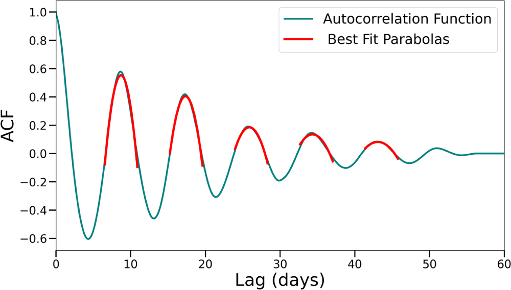
Figure A4. We include comparisons of the  and
and  posteriors for each planet in the system. Batygin & Morbidelli (2013) predict that the argument of periastrons of neighboring planets should be anti-aligned when in resonance. Planets in the TOI-1136 system seem to generally follow this principle, a strong indicator that the system experienced Type I migration.
Download figure:
Standard image High-resolution image
Table A1. TTV-only Posteriors of TOI-1136 b
| Parameter Name | 6p TTV Posterior | Units | Description |
|---|---|---|---|
| Planet b | |||
| Fit Parameters | |||
| Pb | 4.1728 ± 0.0002 | days | Orbital period |

| 0.15 ± 0.02 | ⋯ | Eccentricity reparametrization |

|

| ⋯ | Eccentricity reparametrization |
| Mb |

| degrees | Mean anomaly |
| ib | 86.43 ± 0.27 | degrees | Inclination |
| mp,b |

| M⊕ | Planet mass |
| Derived Parameters | |||
| ρb | 2.71 ± 0.84 | g cc−1 | Bulk density |
| eb | 0.03 ± 0.01 | ⋯ | Eccentricity |
| ωb | 31 ± 7 | degrees | Argument of periastron |
| ab | 0.0511 ± 0.0006 | au | Semimajor axis |
| Teq,b a | 1216 ± 10 | K | Equilibrium temperature |
| Planet c | |||
| Fit Parameters | |||
| Pc | 6.2573 ± 0.0002 | days | Orbital period |

| −0.112
| ⋯ | Eccentricity reparametrization |

| −0.305 ± 0.010 | ⋯ | Eccentricity reparametrization |
| Mc |

| degrees | Mean anomaly |
| ic |

| degrees | Inclination |
| mp,c |

| M⊕ | Planet mass |
| Derived Parameters | |||
| ρc | 1.58 ± 0.19 | g cc−1 | Bulk density |
| ec | 0.11 ± 0.01 | ⋯ | Eccentricity |
| ωc | 70 ± 2 | degrees | Argument of periastron |
| ac | 0.0669 ± 0.0005 | au | Semimajor axis |
| Teq,c | 1062 ± 7 | K | Equilibrium temperature |
| Planet d | |||
| Fit Parameters | |||
| Pd | 12.5200 ± 0.0002 | days | Orbital period |

| −0.100 ± 0.007 | ⋯ | Eccentricity reparametrization |

| 0.093 ± 0.008 | ⋯ | Eccentricity reparametrization |
| Md |

| degrees | Mean anomaly |
| id | 89.4 ± 0.3 | degrees | Inclination |
| mp,d | 9.4 ± 1.2 | M⊕ | Planet mass |
| Derived Parameters | |||
| ρd | 0.41 ± 0.05 | g cc−1 | Bulk density |
| ed | 0.019 ± 0.002 | ⋯ | Eccentricity |
| ωd | −43 ± 3 | degrees | Argument of periastron |
| ad | 0.1062 ± 0.0004 | au | Semimajor axis |
| Teq,d | 843 ± 5 | K | Equilibrium temperature |
| Planet e | |||
| Fit Parameters | |||
| Pe |

| days | Orbital period |

| 0.0825 ± 0.006 | ⋯ | Eccentricity reparametrization |

| −0.184 ± 0.007 | ⋯ | Eccentricity reparametrization |
| Me |

| degrees | Mean anomaly |
| ie | 89.3 ± 0.3 | degrees | Inclination |
| mp,e | 6.8 ± 0.7 | M⊕ | Planet mass |
| Derived Parameters | |||
| ρe | 1.41 ± 0.19 | g cc−1 | Bulk density |
| ee | 0.041 ± 0.003 | ⋯ | Eccentricity |
| ωe | −63.3 ± 1.2 | degrees | Argument of periastron |
| ae | 0.139 ± 0.001 | au | Semimajor axis |
| Teq,e | 736 ± 5 | K | Equilibrium temperature |
| Planet f | |||
| Fit Parameters | |||
| Pf | 26.321 ± 0.0008 | days | Orbital period |

|

| ⋯ | Eccentricity reparametrization |

| −0.013
| ⋯ | Eccentricity reparametrization |
| Mf |

| degrees | Mean anomaly |
| if | 89.4 ± 0.2 | degrees | Inclination |
| mp,f |

| M⊕ | Planet mass |
| Derived Parameters | |||
| ρf | 0.89 ± 0.22 | g cc−1 | Bulk density |
| ef | 0.000 ± 0.001 | ⋯ | Eccentricity |
| ωf | −42.9 ± 30 | degrees | Argument of periastron |
| af | 0.174 ± 0.001 | au | Semimajor axis |
| Teq,f | −658 ± 4 | K | Equilibrium temperature |
| Planet g | |||
| Fit Parameters | |||
| Pg | 39.546 ± 0.001 | days | Orbital period |

|

| ⋯ | Eccentricity reparametrization |

| −0.18 ± 0.01 | ⋯ | Eccentricity reparametrization |
| Mg | −120.5
| degrees | Mean anomaly |
| ig | 89.6 ± 0.2 | degrees | Inclination |
| mp,g |

| M⊕ | Planet mass |
| Derived Parameters | |||
| ρg | 3.77 ± 1.19 | g cc−1 | Bulk density |
| eg | 0.033 ± 0.004 | ⋯ | Eccentricity |
| ωg | −81 ± 2 | degrees | Argument of periastron |
| ag | 0.229 ± 0.001 | au | Semimajor axis |
| Teq,g | 574 ± 4 | K | Equilibrium temperature |
| TOI-1136 (h) |
Notes.
a Estimated using an albedo of 0. b All of the orbital parameters presented in this table are osculating elements computed at BJD 2458680 days.