Energy Distribution Diagram Used for Cost-Effective Battery Sizing of Electric Trucks

Abstract

One possible step for reducing humans’ use of fossil fuel due to transport tasks is to replace diesel trucks with battery electric ones. This paper introduces the energy distribution diagram, which makes it easy to visualise the trucks’ daily energy consumption over their full service life. The energy distribution is used to investigate which driving patterns are suitable for cost-effective battery electric trucks when compared to commercial diesel trucks. It is shown that the battery capacity that results in the lowest cost per kilowatt-hour propulsion energy depends on the driving pattern, and an algorithm for selecting the most cost-effective capacity is presented. In many instances, it was found that battery electric trucks competed favourably with diesel trucks, especially when the trucks had low variations in daily energy consumption. It is beneficial to determine the circumstances under which they may be cheaper, as this will facilitate the transition to battery electric trucks in segments with a reduced overall cost of ownership.

1. Introduction

Society’s dependence on oil is problematic, since calculations show the reserve depletion times are less than 30 years [1] and continued extensive use of fossil fuel will likely have severe consequences for the Earth’s climate system [2]. Other downsides of greenhouse gas emissions, such as pollution and negative health impacts, are also expressed in the literature [3]. An attempt to partly solve this grave problem is to use battery electric trucks instead of diesel ones. Another possible solution is using hydrogen trucks, but recently published studies favour the battery electric type [4,5]. Yet another study declares the promising feasibility of the battery electric trucks, but notes that fuel cells might be better for heavy-duty trucks on extra-long journeys [6]. This paper aims to contribute to the transition from diesel to battery electric trucks. It will do so by introducing a method to help obtain the various important results needed to design cost-effective charging strategies and battery and charger sizes. Cost-efficient solutions for battery electric trucks are vital, as it is assumed they will accelerate the transition from diesel to battery electric trucks. In presenting a systematic review of the cost of battery packs, Nykvist and Nilsson highlight battery price as a crucial parameter for cost-competitive battery electric vehicles [7]. In their article the authors claim (with the support of a previous study [8]), that the price of batteries must fall below 150 $/kWh if battery electric vehicles in general are to compete with internal combustion vehicles. They also show that such a price can be achieved in the near future. The present paper introduces a method facilitating cost comparisons, taking vehicle usage patterns into account. It will be shown that, even at a battery cost of 200 €/kWh, many commercial battery electric trucks will be cost-competitive with diesel trucks. This is because commercial trucks have a high utilisation rate compared to private passenger cars. However, it is worth mentioning that, to be used, battery electric trucks do not necessarily have to be cheaper than diesel ones. They simply have to be the most cost-effective way of replacing fossil fuel transport.

Previous research gives an example of the cost-competitiveness of battery electric against commercial diesel trucks [9] and states that the cost-effectiveness of battery electric vehicles is sensitive to driving patterns [10]. It is subsequently established that relatively uniform driving patterns are favourable to electrification [11]. This paper further investigates the cost-effectiveness of battery electric trucks across a wide variety of driving patterns. Previous studies have used probability density functions for the daily driven distance of battery electric vehicles [10,12]. This paper takes a different approach, basing its analysis on the daily energy consumption of all operating days in a vehicle’s service life. The daily energy consumption in a battery electric truck’s service life is visualised in an energy distribution diagram. The energy distribution includes more information than a probability distribution for the daily distance travelled, but generally allows for similar types of analysis. However, we suggest that the energy distribution diagram is more of a practical tool as it can visualise the information needed to perform the analysis more directly. Moreover, analysing the daily consumed energy instead of the daily distance travelled has the advantage that the outcome can also be useful for battery electric vehicles that do not use all their energy to move; an excavator, for example.

In a previous study of a commercial electric vehicle, a battery-ageing model is used to consider the effects of ageing due to battery size [13]. That study found that an oversized battery could lead to a lower total cost of ownership because it reduced battery ageing. The fact that larger batteries prevent deep battery cycles and thus reduce battery ageing is also stated in another study [14]. Due to the battery ageing and safety margins, this paper assumes that a maximum of 80% of nominal battery capacity can be used. Using vehicle batteries as a means of grid energy storage can reduce the total cost of battery electric vehicles, but this is not included in this paper. This theme has been analysed in such works as [15], which finds that grid storage has only limited value for plug-in hybrids.

A study of electric delivery trucks concluded that battery sizing is essential for maximising profit [16]. However, there is no unambiguous answer to the question of which power train results in the lowest total cost of ownership, as this will depend on how the vehicle is used [17]. This paper investigates cost-efficient battery sizing for different driving patterns with the aim of finding when battery electric trucks are competitive to diesel trucks. From the work done in this paper, it is clear that the energy distribution diagram is a useful tool for determining the most cost-effective battery capacity. The study also indicates that battery electric trucks are competitive with diesel trucks in many different driving patterns. This paper focuses on battery electric trucks, but its analysis is general and can easily be applied to other types of battery electric vehicles by making the right changes to the parameters.

2. Designing Electromobility Systems Using Energy Distribution Diagrams

Finding the best system design for battery electric vehicles is a very complex issue, as many compromises can only be made on a high system level. What may be an improvement in one part of the system (such as a cheaper truck) may lead to drawbacks in a completely different part (such as reduced reliability in the logistics chain). It is, therefore, not possible to build the most cost-effective system by designing all its parts to meet fixed specifications at minimum cost. Because one needs to make such system-level compromises, evaluating which system is the best must be done on a transport system level. This requires domain experts from many different areas to cooperate on finding the best system trade-offs.

However, since the investigated system is so big, with so many different aspects to consider, it will be impossible to carry out a cross-disciplinary system analysis that includes the full complexity of each subsystem. Rather, there is a need to find which aspects of a subsystem are critical to the way the rest of the system is designed and which are not. For the system-level analysis, one must try and find simplified models which can be understood by experts from different domains. They can then link these models to their own domain expertise and draw conclusions that transcend their specialist domain.

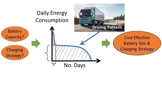
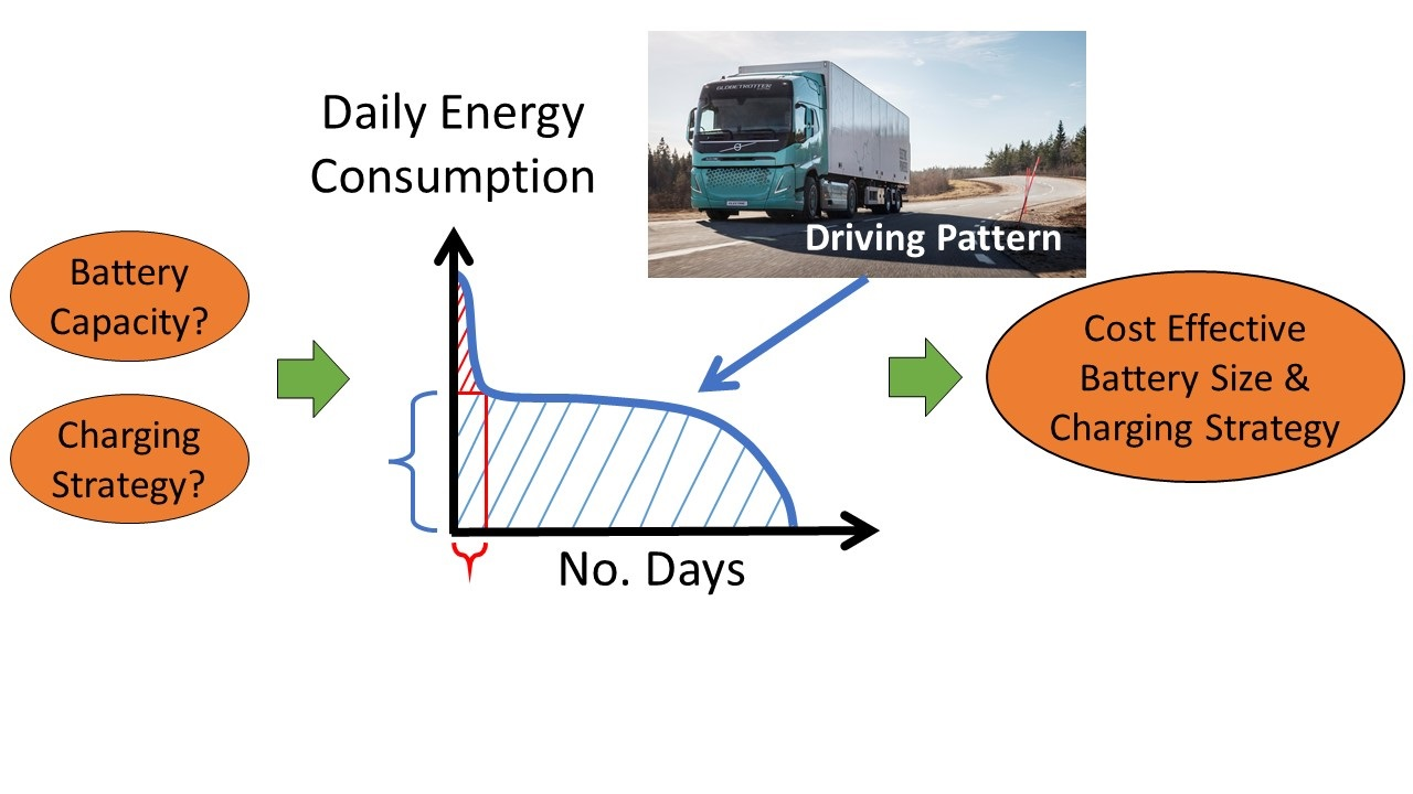
The energy distribution diagram (EDD) is such a tool. It aims to explain important mechanisms linking the usage pattern of a specific vehicle to battery size, charging strategy and total cost of owning the vehicle. Using the EDD, it is possible to understand many important design decisions from the vehicle owner’s perspective. By itself, the EDD cannot tell us what the overall optimal system design is, but it will provide key information to help make system trade-offs. This paper introduces the energy distribution diagram and explains how it can be used to determine several important values. The EDD is also used to find cost-effective battery sizing for some different usage patterns. Note that, in this paper, the analysis is made purely from a vehicle perspective. Thus, what this paper finds to be the cost-effective solution it is not necessarily the same as the optimal solution for the whole system. However, the results still show several very important aspects of battery sizing and these will also be important for the system level.

3. Cost of a Battery Electric Truck

In this analysis, some of the main costs of operating a truck have been assumed to be equal for diesel and battery electric trucks and have thus been omitted from the cost comparisons. This is not because of any limitations when using the EDD to size batteries and estimate charging costs. Rather, the simplification has been made to focus this paper on how the EDD can be used to analyse the effect of varying driving patterns. Costs which this analysis assumes to be equal for both battery and diesel trucks are: the cost of the vehicle (excluding the battery in the electric case), the second-hand value of the vehicle and the cost of maintenance and insurance. Naturally, differences in these costs can influence the cost comparison to some extent. However, it is unclear whether their combined effect will favour electric trucks or diesel ones.

Assuming that trucks are charged during existing driver breaks, the charging will not increase the working hours of the driver. Thus, the driver’s salary also remains the same. Should the charging not be done during driver breaks, the EDD can also provide the number of charging instances and the amount of energy charged from different type of chargers. This makes it possible to estimate the time required for charging and thus any extra driver salary.

Furthermore, this paper assumes that an electric truck can carry the same goods as a diesel truck. This will be true if the goods are not heavy or the driving distance is short (resulting in a small battery). This is the case for most local and regional, as well as some long-haul trucks. So, for them, the results of this analysis are accurate. The main exception is trucks that are driven long distances without charging, in combination with carrying heavy goods. For these, there will be a need to estimate the cost of the reduced payload, and the optimal battery size may be smaller than suggested in this paper.

In this analysis, some costs differ between electric and diesel trucks. These include the fact electric trucks have additional costs for batteries, chargers and grid connection. Additionally, the cost of diesel is replaced with the cost of electricity. In this paper, the costs are normalised and expressed in EUR per kWh of propulsion energy. Whenever the word energy appears in this paper, it stand for propulsion energy. The fuel cost for diesel trucks is estimated at 0.30 €/kWh. This cost is based on a diesel price of 1.2 €/L (excl. VAT) and a high powertrain efficiency of 40%. This cost estimate is low, especially given the recent surge in diesel prices. However, the calculations were made before the strong diesel price increases of 2021 and 2022 and it is not impossible that the current diesel price may only be temporary. Moreover, the authors wanted to be sure that the reference value of diesel was not too high. Based on this price picture, if it can be shown that electric trucks are competitive, then the conclusions should be quite reliable. Thus, for electric trucks to be cost-competitive, the cost of the electricity, battery, grid and charger should not total more than 0.30 €/kWh. A realistic electricity price, excluding grid tariffs, is 0.08 €/kWh when using a privately owned charger. The price of using a public fast charger is uncertain, but around 0.4 €/kWh. The estimated average charge and discharge losses and efficiency of the electric powertrain have been indirectly included, as an increase in the price of the electricity per kWh of propulsion energy. This is similar to the way in which the average efficiency of the diesel powertrain has been included in the cost of diesel. The cost of a complete battery system is set at 200 €/kWh and the battery is assumed to last as long as the truck. In this analysis, the economic life is assumed to be seven years. The price of a charger increases with its power and is about 400 €/kW, the annual grid fee can vary but is around 60 €/kW/year. Even the charger is assumed to have a service life of only seven years, due to the rapid development of the charging technology.

To make the analysis more general, variables for the different costs and their assumed values are introduced in

Table 1. Notations for the different costs and their assumed values. Please keep in mind that the cost refers to the cost of propulsion energy.

Costs	Notation	Typical Value
Diesel Cost	$C_d$	0.30 €/kWh
Electricity Cost, Private Charging	$C_e$	0.08 €/kWh
Electricity Cost, Public Fast Charging	$C_{epub}$	0.4 €/kWh
Battery Cost	$C_b$	200 €/kWh
Price of Charger	$C_{charger}$	400 €/kW
Grid Fee	$C_g$	60 €/kW/year
Service Life of Truck, Charger and Battery	T	7 years
Combined Price of Charger and Grid	$C_{ch}=\frac{C_{charger}}{T}+C_g$	117 €/kW/year

. To make the following equations more readable, a combined parameter for the price of the charger and grid has also been introduced in the table. The combined parameter can be seen as the total cost for the charger depreciation and annual grid fee. This generalisation is advantageous, as the parameter values will probably change with time.

To calculate the cost of operating a truck, one only needs to know a few parameter values for how that truck is used and charged. These include the amount of propulsion energy consumed over the vehicle’s service life, $E_{tot}$ (which applies to both diesel and electric trucks). For the electric trucks, one also needs to know the ratio $r_{ch}$, which is the energy derived from the truck owner’s private charger, divided by the total amount of energy ($E_{tot}$). The cost will also be influenced by the battery capacity $B_c$ and power of the private charger $P_{ch}$. These parameters are summarised in

Table 2. Notations for parameters.

Parameters	Notation
Total Propulsion Energy Consumed Over the Trucks Service Life	$E_{tot}$
Ratio of Private Charging to the Total Amount of Energy	$r_{ch}$
Battery Capacity	$B_c$
Charger Power	$P_{ch}$

.

One aim of this paper is to find solutions for battery electric trucks so that they are cost-competitive with commercial diesel trucks. This means that the total cost for the electric truck should be less than or equal to the cost for a diesel truck. In other words, the sum of the cost per kWh for:

• Energy from private charging;
• Energy from public charging;
• Battery;
• Charger;
• Grid fees;

should be less than or equal to the cost per kWh for diesel. Thus, the following inequality should be satisfied:

$$\begin{array}{c}\hfill r_{ch}·C_e+(1-r_{ch})·C_{epub}+\frac{C_b·B_c}{E_{tot}}+\frac{C_{charger}·P_{ch}}{E_{tot}}+T·\frac{C_g·P_{ch}}{E_{tot}}\le C_d.\end{array}$$

(1)

To make the discussion and calculations clearer, the left-hand side of inequality (1) is expressed as a cost function, $f_{BEV}$, according to:

$$\begin{array}{c}\hfill f_{BEV}=r_{ch}·C_e+(1-r_{ch})·C_{epub}+\frac{C_b·B_c}{E_{tot}}+\frac{C_{charger}·P_{ch}}{E_{tot}}+T·\frac{C_g·P_{ch}}{E_{tot}}\\ \hfill =r_{ch}·C_e+(1-r_{ch})·C_{epub}+\frac{C_b}{\frac{E_{tot}}{B_c}}+\frac{T·P_{ch}}{E_{tot}}\left(\frac{C_{charger}}{T}+C_g\right).\end{array}$$

(2)

Defining the battery utilisation factor, ${\Gamma }_b$, as:

$${\Gamma }_b:=\frac{E_{tot}}{B_c},$$

(3)

the battery utilisation factor has the dimensionless unit equivalent full cycles and describes the number of full discharge cycles that can deliver the total amount of energy consumed. Additionally, the charger utilisation factor ${\Gamma }_{ch}$ is defined as the total energy delivered by the charger over its service life divided by the maximum possible amount of energy that can be delivered from the charger over its service life. The charger utilisation factor is, therefore, a dimensionless scalar with possible values from 0% to 100%. Thus:

$${\Gamma }_{ch}:=\frac{E_{ch}}{T·P_{ch}},$$

(4)

where $E_{ch}$ is the total amount of energy delivered by the charger over its service life. By using the notation for the combined prices for charger and grid according to Table 1 together with $E_{ch}=r_{ch}·E_{tot}$ it is now possible to express the cost function as:

$$f_{BEV}=r_{ch}·C_e+(1-r_{ch})·C_{epub}+\frac{C_b}{{\Gamma }_b}+\frac{r_{ch}·C_{ch}}{{\Gamma }_{ch}}.$$

(5)

The cost parameters in Table 1 will be determined by the market and technology development, while the total energy consumed for a vehicle during its service life will depend on the truck’s transport task. However, the parameters for battery capacity, charger power and ratio of private charging are of special interest, as they will change depending on the charging strategy. As seen from Equation (5), one should aim to choose the battery capacity and charging power so that they increase the utilisation factors, but simultaneously avoid too much public fast-charging, which decreases $r_{ch}$ and therefore increases the cost. If the relationship between these parameters can be expressed, it may be possible to optimise these parameters and determine the lowest total cost per propulsion kWh. This paper will show that the relationship depends on the shape of the energy distribution diagram for the truck. This will be introduced in the next section.

4. The Energy Distribution Diagram

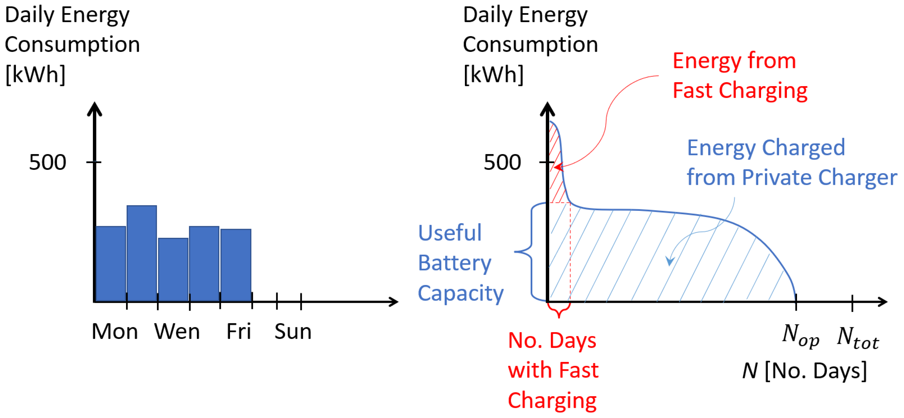
A truck’s daily energy consumption will differ each day due to such things as varying transport tasks and weather conditions. The daily energy consumption data for a truck can be presented in an energy distribution diagram. Consider a truck’s daily energy consumption over a week, as shown in the left-hand part of Figure 1. The length of each bar on the y-axis represents the energy consumed for that day. A truck’s service life consists of many days and, if these are sorted according to energy consumption, starting with the highest figure, a curve is derived. This is called an energy distribution diagram (note that the curve should actually be a discrete number of points, but for convenience, it appears as a continuous curve), see the right-hand part of Figure 1. The total number of days in the vehicle’s service life is $N_{tot}$, and the number of days the vehicle is operational is $N_{op}$. Rearranging the days according to energy consumption does not pose a problem, since the truck is charged at night and thus the energy needs of the coming day are independent of the previous day’s consumption. Sorting the days by energy consumption has advantages. For example, it is easier to read the highest daily energy consumption, or estimate the mean energy consumption. It is also possible to approximate the sorted EDD using a monotonically decreasing mathematical function. Note that for vehicles that are charged after each trip, it is possible to change the x-axis to show the number of trips rather than the number of days.

By plotting the useful battery capacity in the EDD, the number of days can be determined for which the battery is too small to run an entire day on a single charge. On these days, the vehicle will need to fast charge during the day. Assuming that fast charging only adds the minimum energy needed to carry out the rest of the day’s driving, the energy which needs to be fast charged can be determined as the red-striped area in the diagram.

The EDD gives a lot of concentrated information on the full service life of a vehicle. This information is listed below:

• The total energy consumption is the area under the curve.
• The total number of operational days is found from the curve’s intersection with the x-axis.
• The mean consumed energy for the days when the truck is used equals the total energy divided by the number of operational days.
• The highest consumed energy can be read off from the curve’s intersection with the y-axis.
• The number of days that need fast charging and the amount of fast charging needed for a particular useful battery capacity.
• The shape of the EDD gives a quick picture of the size of the variation in daily energy consumption and the respective share of days with high, medium or low energy consumption.

When considering the right-hand part of Figure 1, it may look as though the optimal charging strategy is strongly influenced by the shape of the EDD. For example, can it be a good idea to select a battery capacity that can handle the majority of the trips, but not the slender EDD peak? In that case the battery cost is greatly reduced compared to a battery that can handle all the trips, while only requiring a small amount of public fast charging. Subsequent sections will investigate the most cost-efficient charging strategy for different shapes of EDD, with the aim of finding which EDD shapes give cost-efficient solutions for battery electric trucks. All the analysis is made under the assumption that the battery capacity and power of the charger are continuous variables (spanning from zero to arbitrary high values) and that charging is possible exactly when needed.

5. A Rectangular Energy Distribution Diagram

This section investigates a rectangular EDD, which represents a truck using the same amount of energy each day during its whole service life. Of course real trucks never consume exactly the same energy each day, but it is rather common that trucks are used in very similar ways most days. So, although an extreme case, the rectangular EDD is interesting to study.

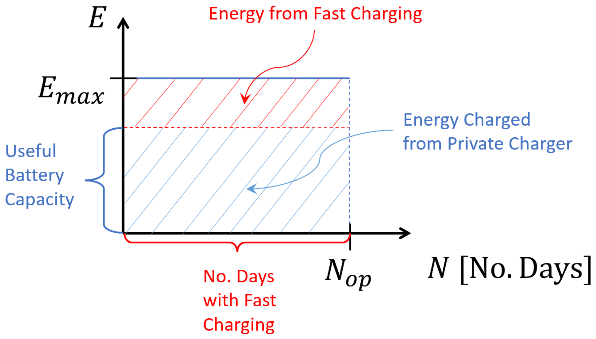
Let $E\left(N\right)$ be the total amount of energy consumed by a truck during day N, i.e., $E\left(N\right)$ describes the EDD’s envelope and is, therefore, called the “energy function”. Let the highest energy consumption for a day be $E_{max}$. Thus, the energy function for a rectangular EDD is given by:

$$E\left(N\right)=E_{max},N\in [0,N_{op}],$$

(6)

where $N_{op}$ is the number of operational days for the truck. This energy function gives a rectangular EDD, see Figure 2.

The most cost-effective battery capacity, charger power and the share of public fast charging will now be determined. Due to battery ageing and safety margins, it is assumed that only a share of the battery capacity, $r_{SoC}$, can be used. This paper assumes that up to 80% of the battery capacity may be used and therefore:

$$r_{SoC}=0.8.$$

(7)

Thus, at the start of a day, the available energy charged during the night is $r_{SoC}·B_c$. The rest, up to $E_{max}$, must be charged at public fast chargers. By dividing the energy charged using the home charger over the truck’s service life by the total energy it uses over its service life, the result is:

$$r_{ch}=\frac{r_{SoC}·B_c}{E_{max}}$$

(8)

or equivalent:

$$B_c=\frac{E_{max}·r_{ch}}{r_{SoC}}$$

(9)

for a rectangular EDD. From the definition of the battery utilisation factor, one obtain:

$${\Gamma }_b=\frac{E_{tot}}{B_c}=\frac{r_{SoC}·E_{tot}}{E_{max}·r_{ch}}.$$

(10)

As one want the cheapest possible charger that can charge the maximum daily energy consumption in one night, the charger power should be:

$$P_{ch}=\frac{r_{SoC}·B_c}{T_{ch}},$$

(11)

where $T_{ch}$ is the time for which the charger can be used every night (the charger runs on full power). The charger utilisation factor can now be expressed as:

$${\Gamma }_{ch}=\frac{E_{ch}}{P_{ch}·T}=\frac{r_{ch}·E_{tot}}{P_{ch}·T}=\frac{r_{ch}·E_{tot}}{\frac{r_{SoC}·B_c}{T_{ch}}·T}=\frac{N_{op}·T_{ch}}{T},$$

(12)

where the last equality is obtained by Equation (8) and the fact that $\frac{E_{tot}}{E_{max}}=N_{op}$ for a rectangular EDD. Using the above equations in Equation (5) produces the following expression of cost function:

$$\begin{array}{c}\hfill f_{BEV}=r_{ch}·C_e+(1-r_{ch})·C_{epub}+\frac{C_b}{\frac{r_{SoC}·E_{tot}}{E_{max}·r_{ch}}}+\frac{r_{ch}·C_{ch}}{\frac{N_{op}·T_{ch}}{T}}\\ \hfill =r_{ch}·C_e+(1-r_{ch})·C_{epub}+\frac{C_b·r_{ch}}{r_{SoC}·N_{op}}+\frac{T·C_{ch}·r_{ch}}{N_{op}·T_{ch}}.\end{array}$$

(13)

The cost function is now expressed as a function solely of the variable $r_{ch}$. Thus, the derivative of $f=f\left(r_{ch}\right)$ is studied in order to find the lowest cost:

$$\frac{d{f}_{BEV}}{d{r}_{ch}}=C_e-C_{epub}+\frac{C_b}{r_{SoC}·N_{op}}+\frac{T·C_{ch}}{N_{op}·T_{ch}}.$$

(14)

By assuming that $T_{ch}=14$ h, $N_{op}=1750$ (corresponds to 5 days per week, 50 weeks per year over 7 years) and inserting the parameter values from Table 1 one obtains:

$$\frac{d{f}_{BEV}}{d{r}_{ch}}<0,$$

(15)

which implies that the lowest cost per kWh has been obtained for the highest possible value of $r_{ch}$ which is $r_{ch}=1.$ Inserting $r_{ch}=1$ in Equation (13) with the same parameter values as previously produces:

$$f_{BEV}\left(1\right)=0.26€/\mathrm{kWh}<C_d.$$

(16)

In this case, the cost for the battery is the largest proportion; 0.14 €/kWh compared to the other costs (cost of electricity from home charging, 0.08 €/kWh, cost of public fast charging, 0 €/kWh and cost of the charger and grid, 0.03 €/kWh). (Due to rounding, the individual costs do not seem to add up to the total cost). Since $r_{ch}=1$ corresponds to charging all the energy at home, it may be concluded that, with the EDD as a rectangle, the most cost-efficient charging strategy is night charge only and that the battery should be sized so that $r_{SoC}·B_c=E_{max}$. In this case, an electric truck will be more cost-efficient than today’s commercial diesel trucks. Note that the total cost is the same, irrespective of the highest energy consumption for a day, but that it reduces if the total number of operational days is increased. Additionally, note that with $r_{ch}=1$, Equation (10) now gives ${\Gamma }_b=r_{SoC}·N_{op}$ since $N_{op}=\frac{E_{tot}}{E_{max}}$ for a rectangular EDD. This is intuitive, since all the useful capacity is used exactly once every day.

6. A Triangular Energy Distribution Diagram

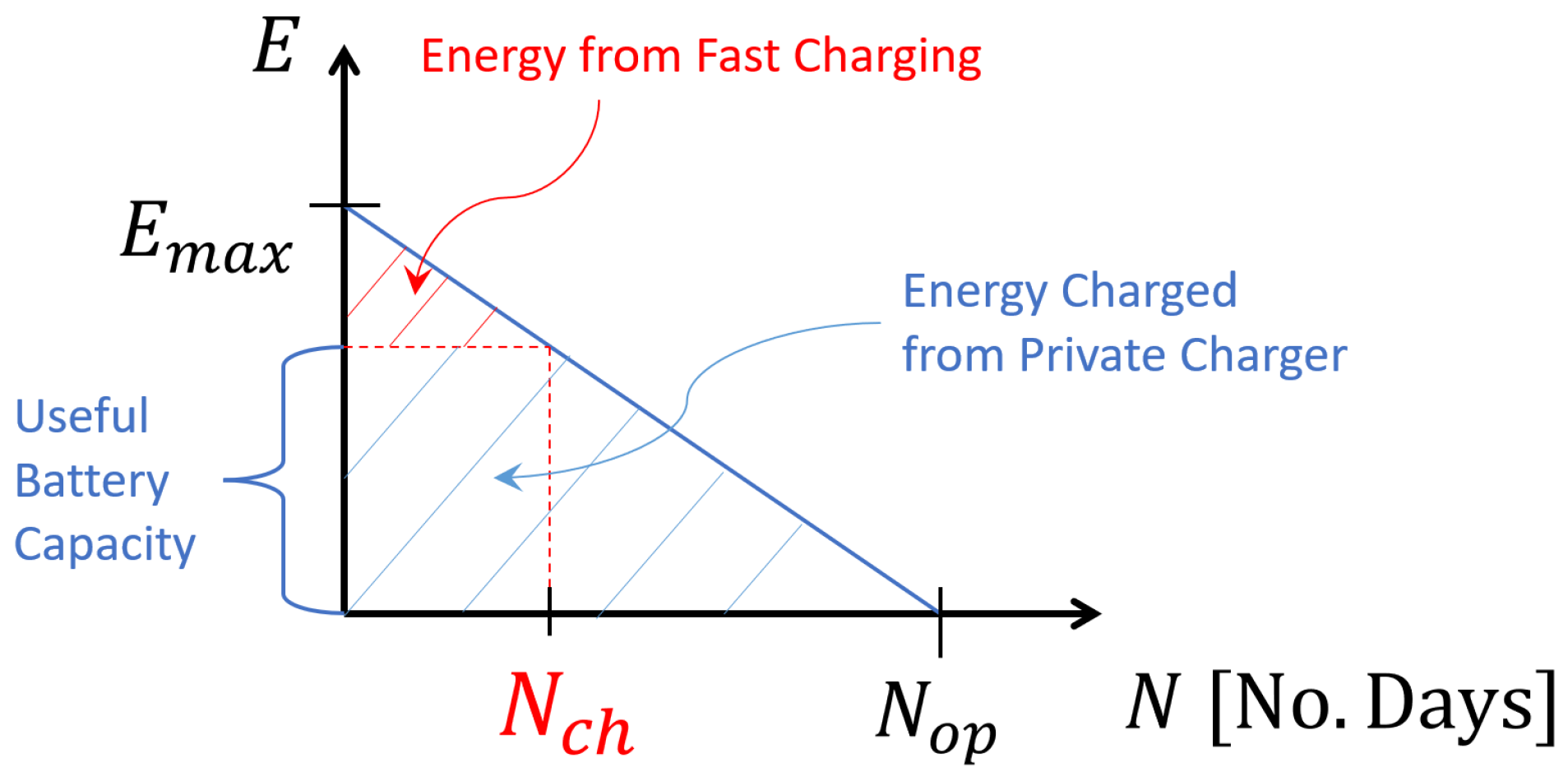
The previous section showed that the charging strategy night charge only was cost-efficient when the EDD was rectangular. A triangular EDD will now be similarly investigated. A triangular EDD represents a truck, which uses different amount of energy each day, between zero and a maximum value $E_{max}$ and all the levels of daily energy consumption are equally common. This is an unusual way of using a truck, but is interesting to study as it results in a more difficult trade-off when selecting battery capacity. The triangular energy function can be expressed as:

$$E\left(N\right)=-\frac{E_{max}}{N_{op}}N+E_{max},N\in [0,N_{op}].$$

(17)

The energy function is illustrated in Figure 3. In the figure, the available energy stored in a full battery is marked in blue on the y-axis and the number of days charging with a public fast charger is marked in a red $N_{ch}$ on the x-axis.

The aim is to find the battery capacity that gives the lowest value on the cost function. Therefore, the cost function will be expressed solely as a function of battery capacity and the parameters. The mathematical steps follow below. Figure 3 makes it apparent that the amount of energy to be charged by public chargers corresponds to the area of the small upper triangle of height $E_{max}-r_{SoC}·B_c$ and base $N_{ch}$, with the rest charged at night using a private charger. Thus:

$$r_{ch}=\frac{\frac{E_{max}·N_{op}}{2}-\frac{(E_{max}-r_{SoC}·B_c)·N_{ch}}{2}}{\frac{E_{max}·N_{op}}{2}}=1-\frac{(E_{max}-r_{SoC}·B_c)·N_{ch}}{E_{max}·N_{op}}.$$

(18)

To eliminate $N_{ch}$, Equation (17) and Figure 3 can be used, thus:

$$-\frac{E_{max}}{N_{op}}·N_{ch}+E_{max}=r_{SoC}·B_c\iff N_{ch}=\frac{(E_{max}-r_{SoC}·B_c)·N_{op}}{E_{max}}$$

(19)

This gives:

$$r_{ch}=1-\frac{(E_{max}-r_{SoC}·B_c)·\frac{(E_{max}-r_{SoC}·B_c)·N_{op}}{E_{max}}}{E_{max}·N_{op}}=1-{\left(1-\frac{r_{SoC}·B_c}{E_{max}}\right)}^2.$$

(20)

Again, the definition of the battery utilisation factor is:

$${\Gamma }_b=\frac{E_{tot}}{B_c}$$

(21)

and for the triangular EDD, the charger utilisation factor becomes:

$$\begin{array}{c}\hfill {\Gamma }_{ch}=\frac{E_{ch}}{P_{ch}·T}=\frac{r_{ch}·E_{tot}}{P_{ch}·T}=\frac{r_{ch}·\frac{E_{max}·N_{op}}{2}}{\frac{r_{SoC}·B_c}{T_{ch}}·T}=\frac{r_{ch}}{\frac{r_{SoC}·B_c}{E_{max}}·\frac{2·T}{N_{op}·T_{ch}}}.\end{array}$$

(22)

By inserting Equations (20)–(22) in Equation (5), one obtains:

$$\begin{array}{c}\hfill f_{BEV}=\left(1-{\left(1-\frac{r_{SoC}·B_c}{E_{max}}\right)}^2\right)·C_e+\left(1-\left[1-{\left(1-\frac{r_{SoC}·B_c}{E_{max}}\right)}^2\right]\right)·C_{epub}\\ \hfill +\frac{C_b·B_c}{E_{tot}}+\frac{r_{ch}}{\frac{r_{ch}}{\frac{r_{SoC}·B_c}{E_{max}}·\frac{2·T}{N_{op}·T_{ch}}}}·C_{ch}\\ \hfill =\left(1-{\left(1-\frac{r_{SoC}·B_c}{E_{max}}\right)}^2\right)·C_e+{\left(1-\frac{r_{SoC}·B_c}{E_{max}}\right)}^2·C_{epub}\\ \hfill +\frac{C_b}{r_{SoC}·\frac{N_{op}}{2}}·\frac{r_{SoC}·B_c}{E_{max}}+\frac{r_{SoC}·B_c}{E_{max}}·\frac{2·T}{N_{op}·T_{ch}}·C_{ch}.\end{array}$$

(23)

For a clearer view, the substitution:

$$x=\frac{r_{SoC}·B_c}{E_{max}},x\in [0,1]$$

(24)

is made. This gives:

$$\begin{array}{c}\hfill f_{BEV}=\left(1-{\left(1-x\right)}^2\right)·C_e+{\left(1-x\right)}^2·C_{epub}+\frac{C_b}{r_{SoC}·\frac{N_{op}}{2}}·x+\frac{2·T}{N_{op}·T_{ch}}·C_{ch}·x\\ \hfill =(C_{epub}-C_e)·x^2+\left(2·C_e-2·C_{epub}+\frac{C_b}{r_{SoC}·\frac{N_{op}}{2}}+\frac{2·T}{N_{op}·T_{ch}}·C_{ch}\right)·x+C_{epub}.\end{array}$$

(25)

Note that $x=0$ corresponds to $B_c=0$, which is not possible in reality. From the known properties of quadratic functions, one knows that the cost function has a global minimum for x, so that:

$$\frac{d{f}_{BEV}}{dx}=0.$$

(26)

One must therefore solve the equation:

$$2·(C_{epub}-C_e)·x+2·C_e-2·C_{epub}+\frac{C_b}{r_{SoC}·\frac{N_{op}}{2}}+\frac{2·T}{N_{op}·T_{ch}}·C_{ch}=0$$

(27)

which is equivalent to:

$$x=-\frac{2·C_e-2·C_{epub}+\frac{C_b}{r_{SoC}·\frac{N_{op}}{2}}+\frac{2·T}{N_{op}·T_{ch}}·C_{ch}}{2·(C_{epub}-C_e)}.$$

(28)

By inserting parameter values from Table 1, $N_{op}=1750$ and $T_{ch}=14$ h one obtain:

$$x=0.45\in [0,1]$$

(29)

and the corresponding minimum cost:

$$\min \left(f_{BEV}\right)=0.34€/\mathrm{kWh}>C_d.$$

(30)

By computing $r_{ch}$ and the utilisation factors, the individual costs can be worked out using Equation (5) (be careful with the units). It becomes apparent that the battery still represents the largest cost, 0.13 €/kWh, closely followed by the cost of public fast charging, 0.12 €/kWh, and that the price for home charging is 0.06 €/kWh. The smallest cost is the charger and grid, at 0.03 €/kWh.

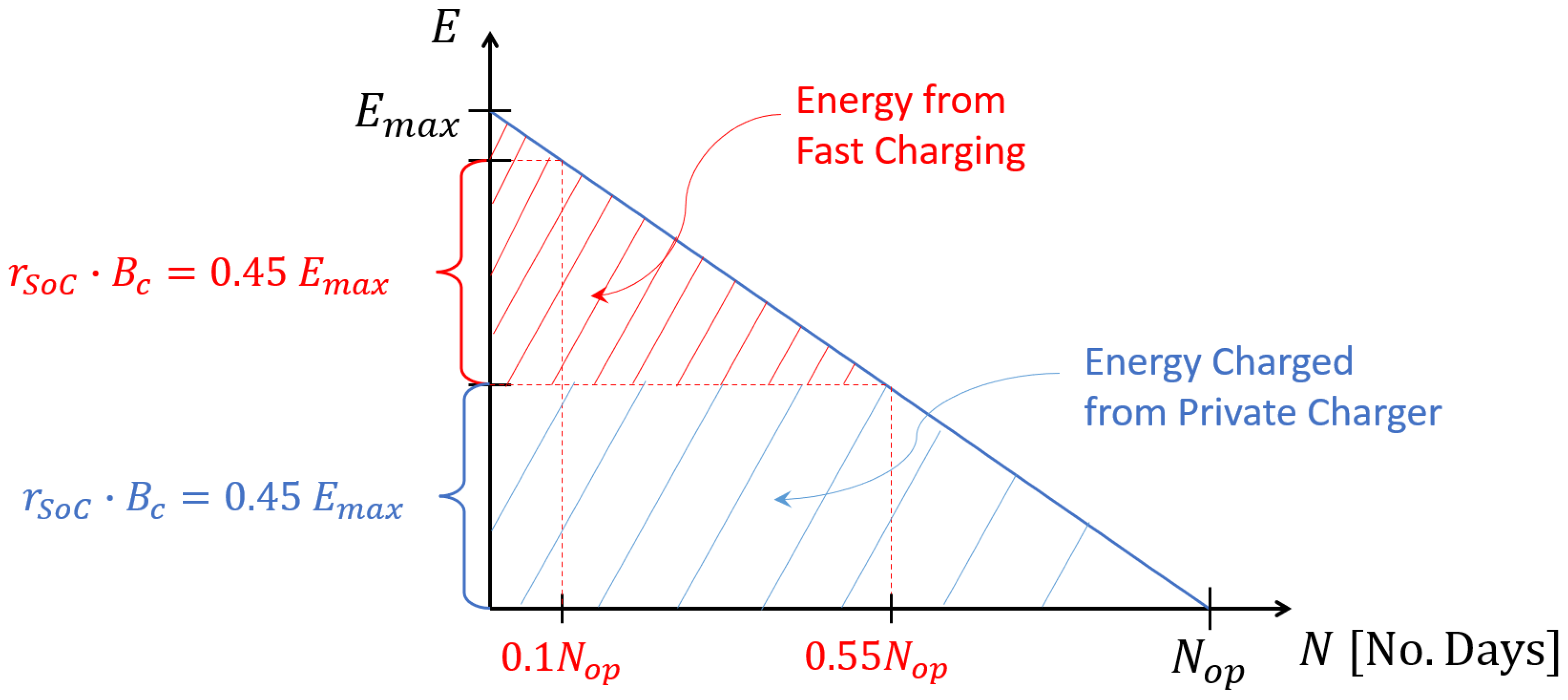
So, if the EDD is triangular, an electric truck has a higher cost per propulsion kWh compared with that of a diesel truck. The battery capacity should be selected so that the useful battery capacity equals 45% of the maximum daily energy consumption. In that case, the cost per propulsion kWh of the electric truck is a little higher than for the diesel truck. Note that (as with the rectangular EDD) the number of operational days influence the result, while the daily maximum consumed energy does not.

A battery sized so that the useful battery capacity equals 45% of the maximum daily energy consumption implies that the truck must charge with public fast chargers on 55% of the days and that it must fast charge twice during the same day on 10% of the days. This is illustrated in Figure 4.

Although this is the most cost-efficient charging strategy, it can lead to inconvenience and operational reliability problems. Luckily, for real commercial trucks, a triangular EDD is rare.

7. A Two-Step Rectangular Energy Distribution Diagram

Imagine an EDD with a thin peak, like the one in the right-hand part of Figure 1. In this case, one might surmise that it will be cost-efficient to size the battery to handle most trips, but not those with the highest energy consumption. Naturally, this strategy will require public fast charging. However, it allows a smaller, cheaper battery. This section will explore how thin the peak must be before it is cost-effective to use fast charging to handle peak demand rather than sizing the battery to fit the peak. To investigate this, a two-step rectangular EDD is analysed. Such an EDD would correspond to a truck being used for two different tasks, different days. Each task consumes exactly the same energy all times it is performed, but the two tasks consumes different energy than each other. Additionally, the number of days which the two tasks are performed can vary. The two-step rectangular EDD appears in Figure 5 and the corresponding energy function can be expressed as:

$$E\left(N\right)=\{\begin{array}{cc}{E}_{max},\hfill & N\in [0,M]\hfill \\ E_{min},\hfill & N\in (M,N_{op}],\hfill \end{array}$$

(31)

where $E_{min}$ is the lowest daily energy consumption for the truck and M is the number of days the truck consumes the maximum daily energy $E_{max}$.

Since the energy function is discontinuous at $N=M$, the calculations needed to determine the most cost-efficient battery capacity are made in two steps. Firstly, it is assumed that $r_{SoC}·B_c\le E_{min}$, which leads to:

$$r_{ch}=\frac{r_{SoC}·B_c·N_{op}}{E_{tot}}$$

(32)

and the battery utilisation factor becomes:

$${\Gamma }_b=\frac{E_{tot}}{B_c}=\frac{r_{SoC}·N_{op}}{r_{ch}}$$

(33)

with the charger utilisation factor:

$${\Gamma }_{ch}=\frac{E_{ch}}{P_{ch}·T}=\frac{r_{ch}·E_{tot}}{P_{ch}·T}=\frac{r_{ch}·E_{tot}}{\frac{r_{SoC}·B_c}{T_{ch}}·T}=\frac{N_{op}·T_{ch}}{T}.$$

(34)

By inserting the expressions of the utilisation factors into Equation (5) one obtain:

$$f_{BEV}=r_{ch}·C_e+(1-r_{ch})·C_{epub}+\frac{C_b}{r_{SoC}·N_{op}}·r_{ch}+\frac{r_{ch}·T}{N_{op}·T_{ch}}·C_{ch},$$

(35)

which is the same equation as Equation (13). One thus obtains the lowest value on $f_{BEV}$ again by taking the highest possible value on $r_{ch}$ which, in this case, is $r_{ch}=\frac{E_{min}·N_{op}}{E_{tot}}$. One concludes that the battery should be sized to handle the low-energy-consumption trips without day charging. The results may seem intuitive after studying the rectangular EDD.

Secondly, consider the case when $r_{SoC}·B_c>E_{min}$. This means that:

$$r_{ch}=\frac{E_{min}·N_{op}+(r_{SoC}·B_c-E_{min})·M}{E_{tot}}.$$

(36)

The charger utilisation factor becomes:

$${\Gamma }_{ch}=\frac{E_{ch}}{P_{ch}·T}=\frac{r_{ch}·E_{tot}}{P_{ch}·T}=\frac{r_{ch}·E_{tot}}{\frac{r_{SoC}·B_c}{T_{ch}}·T}=\frac{r_{ch}·E_{tot}·T_{ch}}{r_{SoC}·B_c·T}.$$

(37)

Inserting this charger utilization factor and the definition of the battery utilisation factor into Equation (5), the cost function becomes:

$$f_{BEV}=r_{ch}·C_e+(1-r_{ch})·C_{epub}+\frac{C_b·B_c}{E_{tot}}+\frac{r_{SoC}·B_c·T}{E_{tot}·T_{ch}}·C_{ch}.$$

(38)

Equation (36) gives:

$$\frac{d{r}_{ch}}{d{B}_c}=\frac{r_{SoC}·M}{E_{tot}}$$

(39)

and therefore:

$$\begin{array}{c}\hfill \frac{d{f}_{BEV}}{d{B}_c}=\frac{r_{SoC}·M}{E_{tot}}·C_e-\frac{r_{SoC}·M}{E_{tot}}·C_{epub}+\frac{C_b}{E_{tot}}+\frac{r_{SoC}·T}{E_{tot}·T_{ch}}·C_{ch}\\ \hfill =\frac{r_{SoC}}{E_{tot}}\left(\frac{C_b}{r_{SoC}}+\frac{T}{T_{ch}}·C_{ch}-(C_{epub}-C_e)·M\right).\end{array}$$

(40)

It appears that the sign of the derivative depends on the parameter M. One can see that:

$$M>\frac{\frac{C_b}{r_{SoC}}+\frac{T}{T_{ch}}·C_{ch}}{C_{epub}-C_e}\iff \frac{d{f}_{BEV}}{d{B}_c}<0$$

(41)

and by inserting the same values as before, one obtains:

$$M>964\iff \frac{d{f}_{BEV}}{d{B}_c}<0.$$

(42)

This means that it becomes cost-efficient to have a smaller battery, one that can handle only the energy needs of low-consumption days, if there are fewer than or equal to 964 days of high energy consumption. The remaining days require fast charging. In other words, it is cost-effective to have a battery that can handle all trips using night charge only if the number of high-consumption days is greater than 964 (note that this is valid for the parameter values selected in this paper). The results confirm the intuition that when an EDD has a peak, it is cost-efficient to have a smaller battery and fast charge the remaining days, but only if the peak is sufficiently thin.

It is now clear how the battery should be sized, but is this electric truck competitive compared to a diesel truck? To investigate this, the cost function is expressed as a function of two variables as follows. Firstly, consider the case when $M\le 964$, which implies that the smaller battery should be chosen. Thus, $r_{SoC}·B_c=E_{min}$, which gives:

$$\begin{array}{c}\hfill r_{ch}=\frac{E_{min}·N_{op}}{E_{tot}}=\frac{E_{min}·N_{op}}{E_{min}·N_{op}+M·(E_{max}-E_{min})}=\frac{r·N_{op}}{r·N_{op}+M·(1-r)}\end{array}$$

(43)

where $r=\frac{E_{min}}{E_{max}}\in [0,1]$. Inserting Equations (33) and (34) into Equation (5) gives:

$$f_{BEV}(M,r)=r_{ch}·C_e+(1-r_{ch})·C_{epub}+r_{ch}·\frac{C_b}{r_{SoC}·N_{op}}+r_{ch}·\frac{T}{N_{op}·T_{ch}}·C_{ch}.$$

(44)

Note that $f_{BEV}=f_{BEV}(M,r)$ since $r_{ch}=r_{ch}(M,r)$.

Secondly, consider the case when $M>964$ and thus $r_{SoC}·B_c=E_{max}$, which gives $r_{ch}=1$, and by Equation (5) one obtains:

$$f_{BEV}=C_e+\frac{C_b}{{\Gamma }_b}+\frac{1}{{\Gamma }_{ch}}·C_{ch}.$$

(45)

The battery utilisation factor then becomes:

$$\begin{array}{c}\hfill {\Gamma }_b=\frac{E_{tot}}{B_c}=\frac{r_{SoC}·E_{tot}}{E_{max}}=\frac{r_{SoC}·(E_{min}·N_{op}+M·(E_{max}-E_{min}))}{E_{max}}\\ \hfill =r_{SoC}·(r·N_{op}+M·(1-r))\end{array}$$

(46)

and the charger utilisation factor is obtained from Equation (37):

$$\begin{array}{c}\hfill {\Gamma }_{ch}=\frac{r_{ch}·E_{tot}·T_{ch}}{r_{SoC}·B_c·T}=\frac{(E_{min}·N_{op}+M·(E_{max}-E_{min}))·T_{ch}}{E_{max}·T}\\ \hfill =\frac{(r·N_{op}+M·(1-r))·T_{ch}}{T}.\end{array}$$

(47)

The above expressions of the utilisation factors give:

$$\begin{array}{c}\hfill f_{BEV}(M,r)=C_e+\frac{C_b}{r_{SoC}·(r·N_{op}+M·(1-r))}+\frac{T}{(r·N_{op}+M·(1-r))·T_{ch}}·C_{ch}.\end{array}$$

(48)

Equations (44) and (48) allow the cost function to be visualised. This is shown in the left-hand part of Figure 6, in which the electric truck is more costly than the diesel truck between the red curve and the M-axis. So, for which type of two-step rectangle EDD is the electric truck competitive with the diesel truck? According to the left-hand part of Figure 6, it is often possible to compete with diesel, but this becomes hard when the EDD is L-shaped. In this case, the spike must be really thin if the cost is not to be too high according to the lower left-hand part of Figure 6. It is also problematic when none of the sides of any rectangle are thin (see centre of left-hand part of Figure 6). Finally, it is problematic when none of the sides of the left-hand rectangle are thin, but the height of the right-hand rectangle is small (like a thin tail). See the lower centre of the left-hand part of Figure 6. The right-hand part of Figure 6 shows how the shape of the two rectangle EDDs depend on M and r. For the shapes of the EDD inside the area enclosed by the red curve and the M-axis, it is hard to compete with the diesel trucks. Note that this area should not be seen as absolutely fixed, especially not those parts close to the red curve, since the area depends on the values of many estimated parameters. The vertical, dashed black line, $M=964$, in the right-hand part of Figure 6 shows how to select battery capacity. On or to the left of the black dashed line, the smaller battery should be selected and, to the right of it, the larger battery.

As seen from Figure 6, the cases when EDDs tend to be a rectangle, or a rectangle with a thin spike are best suited to battery electric trucks. Note that the same cost function value (0.26 €/kWh) is obtained when the two rectangles tend towards forming a single rectangle, as obtained for the rectangular EDD. The cases when the EDD is L-shaped with a really thin spike or when none of the sides of any rectangle are thin show when the electric trucks could compete with diesel trucks. As a rough guide, the closer one gets to the point $(M=750,r=0)$, the harder it is for electric trucks to be competitive, compared with the left-hand part of Figure 6.

From the left-hand part of Figure 6 and the studies of the rectangular EDD, the expectation might be for the rectangular EDD to give the lowest cost per propulsion kWh compared to any EDD for a fixed number of operational days. There now follows a series of arguments showing that a rectangular EDD gives the lowest cost function value.

Take a non-rectangular EDD. The analysis starts by considering the unrealistic case of the battery capacity being zero. The cost function then has the value of $C_{epub}=0.4€/\mathrm{kWh}>f_{BEV}^{rec}$, where $f_{BEV}^{rec}=0.26$ €/kWh is the cost function value when the EDD is rectangular. To try to find a lower cost function value, the battery capacity is increased and, if an EDD is found that is better than the rectangular one, the cost function must begin to drop at some point as battery capacity increases. That being the case, the cost drops because the benefit of charging the majority of the total energy with a home charger rather than a fast public one exceeds the increasing costs of battery, charger, and grid. The required power for the charger is directly proportional to the battery capacity. This means that the extra cost for the battery, charger and grid is the same for any EDD (even the rectangular one) when increasing the battery capacity by a given step according to Equation (2), while the increase in energy that can be moved from public fast charging to home charging is greatest when the EDD is rectangular. Since this maximum decrease in the cost function continues right up until the battery capacity reaches the highest possible value (assuming the battery size is no larger than it needs to manage the trip at the highest daily level of energy consumption), the rectangular EDD must be the most cost-efficient EDD provided the number of operational days is fixed. Or, more simply and less stringently, when the battery size increases, the extra cost of the battery, charger and grid increases equally, independently of the shape of the EDD. However, the most energy will be moved from public fast charging to home charging if the EDD is rectangular. Thus, a rectangular EDD will result in the lowest cost function provided the number of operational days is fixed.

8. Importance of the Number of Operational Days

So far, the number of operational days has been fixed at 1750. However, from the equations, it is apparent that the number of operational days often influences the result. Naturally, if the number of operational days is too low, this makes it impossible for battery electric trucks to compete with commercial diesel trucks because the utilisation factors will be very low. Thus, it is interesting to investigate the lowest necessary number of operational days for battery electric trucks to be competitive. Since the aim is to find a lower bound for the number of operational days, the most preferable EDD is used—the rectangular one. Firstly, from Equation (14), it is clear that:

$$\frac{d{f}_{BEV}}{d{r}_{ch}}<0\iff N_{op}>\frac{\frac{C_b}{r_{SoC}}+\frac{T·C_{ch}}{T_{ch}}}{C_{epub}-C_e}$$

(49)

for a rectangular EDD and by inserting the previous values, one obtains:

$$\frac{d{f}_{BEV}}{d{r}_{ch}}<0\iff N_{op}>964.$$

(50)

Note the similarity with Equations (41) and (42). This means that, if the number of operational days is 964 or less, the lowest value of $r_{ch}$, i.e., $r_{ch}=0$, should be chosen. This gives the lowest cost function value, which would be $C_{epub}=0.4$€/kWh. So, in this case, the battery electric truck is not competitive. Furthermore, in this context, $r_{ch}=0$ corresponds to having a battery capacity of zero kWh, something which is not possible in reality. Thus, one now knows that the number of operational days must be greater than 964, which implies that $r_{ch}=1$.

Secondly, the minimum number of operational days will be determined by solving the inequality:

$$f_{BEV}\left(N_{op}\right)\le C_d.$$

(51)

Equation (13) with $r_{ch}=1$ gives:

$$N_{op}\ge \frac{\frac{C_b}{r_{SoC}}+\frac{T·C_{ch}}{T_{ch}}}{C_d-C_e}$$

(52)

and by inserting the typical values, one obtains:

$$N_{op}\ge 1402.$$

(53)

This means that the number of operational days must be at least 1400 if a battery electric truck is to compete with diesel trucks. This corresponds to approximately five-and-a-half years if the truck is used every weekday. This is exceeded in most commercial trucks.

9. An Algorithm for Sizing the Battery of a General EDD

So far, the most cost-efficient battery size has been determined for a few specific EDD shapes. These cases approximate most of the possible EDDs and give insights as to which EDD shapes are best suited to electric trucks. However, for a specific EDD, it may be necessary to determine the most cost-efficient battery size of that particular EDD rather than just the best battery size for an approximation of it.

As mentioned earlier, three parameters can change when the charging strategy is changed. These are: $B_c$, $r_{ch}$ and $P_{ch}$. This is apparent from Equation (2). However, based on the analysis so far, it is apparent that the three parameters are strongly connected. Since the aim is to use the home charger as much as possible for a given battery capacity and to have a charger powerful enough to supply the full capacity in one night (but no more than that), the choice of $B_c$ directly determines $r_{ch}$ and $P_{ch}$. Thus, a battery capacity may be chosen which determines $r_{ch}$ and $P_{ch}$ and the corresponding cost function value. By systematically testing enough battery capacity values, the most cost-efficient battery capacity can be selected. The most cost-efficient battery capacity will depend on the energy function. This insight allows us to establish an algorithm to determine the most cost-efficient battery capacity for an EDD of arbitrary energy function $E\left(N\right)$. The algorithm follows below.

Algorithm Description

• Choose a sufficiently small battery capacity value, such as $B_{c1}$.
• Compute the total energy, $E_{tot}=\underset{0}{\overset{N_{op}}{\int }}E\left(N\right)dN$.
• Find the smallest $N_1$ so that $r_{SoC}·B_{c1}=E\left(N_1\right)$. The number of days needed to fast charge is $N_1$.
• Compute

  (a)

  $r_{ch}=\frac{r_{SoC}·B_{c1}·N_1+\underset{N_1}{\overset{N_{op}}{\int }}E\left(N\right)dN}{E_{tot}}$,

  (b)

  ${\Gamma }_b=\frac{E_{tot}}{B_{c1}}$

  and

  (c)

  ${\Gamma }_{ch}=\frac{r_{ch}·E_{tot}}{\frac{r_{SoC}·B_{c1}}{T_{ch}}·T}$.

• Compute $f_{BEV1}=f\left(B_{c1}\right)$ from Equation (5).
• Set $B_{c2}=B_{c1}+\Delta B_c$,  $\Delta B_c$ should be sufficiently small.
• Repeat steps 3–6 but increase each index by one until $r_{SoC}·B_{c(n+1)}>E_{max}$, then set $r_{SoC}·B_{c(n+1)}=E_{max}$, repeat steps 3–5 and then jump to step 8.
• One now have the cost per kWh of useful energy expressed as a function of battery capacity. Select the battery capacity that gives the lowest cost.

10. Conclusions

This paper demonstrates that an energy distribution diagram is an effective tool for describing the usage pattern of a vehicle and making it easy to analyse the cost-effectiveness of battery electric vehicles. An algorithm has been presented for determining a cost-effective battery size, charger power and amount of public charging using just the EDD and some cost parameters. This paper focuses on battery electric trucks, but the method could also be used for other battery electric vehicles by making appropriate changes to the parameter values.

How Usage Pattern Influences the Cost-Effectiveness of Battery Electric Vehicles

A rectangular EDD (with no variation in daily energy consumption) gives the lowest cost per kWh propulsion energy compared to all other possible EDDs, for a fixed number of operational days. This is due to making the greatest use of private chargers and no need for fast charging without having an unnecessarily large battery. In this case, night charging only will be the most cost-effective charging strategy. When an EDD is rectangular and has 1750 operating days, an electric truck clearly competes with a diesel truck. However, given the assumed cost parameters, if the number of operational days is fewer than 1400, the diesel truck will cost less.

A triangular EDD leads to a higher total cost than a rectangular one. This is because there is no battery size which can lead to a high level of battery utilisation without also requiring a lot of public fast charging—and vice versa.

In the case of a two-step rectangular EDD, in many of the cases electric trucks can compete with diesel ones. With this EDD, the lowest cost is obtained either by having a battery so large that it can handle all trips without fast charging, or one that can handle solely the low-consumption trips without fast charging. If there are sufficiently many high-consumption days, the large battery should be chosen; otherwise, the choice should be the small one. In this context, “sufficient” means just under 1000 days. The EDDs best suited to electric trucks are those close to a single rectangle, or a rectangle with a thin peak on top. The worst EDDs are L-shaped ones (if their peak is not really thin) and EDDs with a long, thin tail.

For any EDD, provided the shape is fixed, the total cost is reduced by increasing the number of operational days while the maximum daily energy consumption is not influencing the cost.

These conclusions are drawn under the following assumptions:

• Battery capacity and charger power are continuously variable, from zero to arbitrary high values.
• Charging is always possible, precisely when needed.
• Charging is done on planned breaks and requires no extra time.
• A battery electric truck has the same payload capacity as a diesel truck.
• Parameter values are selected according to Table 1, the vehicle is operated for 1750 days, the home charger can be used for up to 14 hours per night and there is 80% of the battery capacity available.

Some of these assumptions are not always true for real trucks. However, the results still allow an increased understanding of how cost-efficiency and charging strategy depend on how a vehicle is used. Typically, the assumptions are reasonable for local trucks and most regional trucks, if they are not carrying very heavy goods or driving very long daily distances. These assumptions favour the battery electric trucks over diesel trucks. However, it should be borne in mind that the price picture will likely change to favour electric trucks as the production volume increases. Additionally, the assumed fuel cost for diesel trucks is intentionally low. Even without these assumptions, the EDD is still a useful tool for determining the cost-effectiveness of battery electric trucks.

References

- Shafiee, S.; Topal, E. When will fossil fuel reserves be diminished? Energy Policy 2009, 10, 181–189. [Google Scholar] [CrossRef]
- IPCC. Climate Change 2021: The Physical Science Basis; Masson-Delmotte, V., Zhai, P., Pirani, A., Connors, S.L., Péan, C., Berger, S., Caud, N., Chen, Y., Goldfarb, L., Gomis, M.I., et al., Eds.; Contribution of Working Group I to the Sixth Assessment Report of the Intergovernmental Panel on Climate Change; Cambridge University Press: Cambridge, UK; New York, NY, USA, 2021; p. 2391. [Google Scholar] [CrossRef]
- Cunanan, C.; Tran, M.-K.; Lee, Y.; Kwok, S.; Leung, V.; Fowler, M. A Review of Heavy-Duty Vehicle Powertrain Technologies: Diesel Engine Vehicles, Battery Electric Vehicles, and Hydrogen Fuel Cell Electric Vehicles. Clean Technol. 2021, 3, 474–489. [Google Scholar] [CrossRef]
- Plötz, P. Hydrogen technology is unlikely to play a major role in sustainable road transport. Nat. Electron. 2022, 5, 8–10. [Google Scholar] [CrossRef]
- Burke, A.; Sinha, A.K. Technology, Sustainability, and Marketing of Battery Electric and Hydrogen Fuel Cell Medium-Duty and Heavy-Duty Trucks and Buses in 2020–2040. In A Research Reportfrom the National Center for Sustainable Transportation; National Center for Sustainable Transportation: Davis, CA, USA, 2020. [Google Scholar]
- Samet, M.J.; Liimatainen, H.; van Vliet, O.P.R.; Pöllänen, M. Road Freight Transport Electrification Potential by Using Battery Electric Trucks in Finland and Switzerland. Energies 2021, 14, 823. [Google Scholar] [CrossRef]
- Nykvist, B.; Nilsson, M. Rapidly falling costs of battery packs for electric vehicles. Nat. Clim. Chang. 2015, 5, 329–332. [Google Scholar] [CrossRef]
- Gaines, L.; Cuenca, R. Costs of Lithium-Ion Batteries for Vehicles; United States Department of Energy: Washington, DC, USA, 2000.
- Moll, C.; Plötz, P.; Hadwich, K.; Wietschel, M. Are Battery-Electric Trucks for 24-Hour Delivery the Future of City Logistics?—A German Case Study. World Electr. Veh. J. 2020, 11, 16. [Google Scholar] [CrossRef] [Green Version]
- Neubauer, J.; Brooker, A.; Wood, E. Sensitivity of battery electric vehicle economics to drive patterns, vehicle range. J. Power Sources 2012, 209, 269–277. [Google Scholar] [CrossRef]
- Hovi, I.B.; Pinchasik, D.; Figenbaum, E.; Thorne, R. Experiences from Battery-Electric Truck Users in Norway. World Electr. Veh. J. 2019, 11, 5. [Google Scholar] [CrossRef] [Green Version]
- Jakobsson, N.; Gnann, T.; Plötz, P.; Sprei, F.; Karlsson, S. Are multi-car households better suited for battery electric vehicles?—Driving patterns and economics in Sweden and Germany. Transp. Res. Part C Emerg. Technol. 2016, 65, 1–15. [Google Scholar] [CrossRef]
- Babin, A.; Rizoug, N.; Mesbahi, T.; Boscher, D.; Hamdoun, Z.; Larouci, C. Total Cost of Ownership Improvement of Commercial Electric Vehicles Using Battery Sizing and Intelligent Charge Method. IEEE Trans. Ind. Appl. 2017, 54, 1691–1700. [Google Scholar] [CrossRef]
- Lunz, B.; Walz, H.; Sauer, D.U. Optimizing vehicle-to-grid charging strategies using genetic algorithms under the consideration of battery aging. In Proceedings of the 2011 IEEE Vehicle Power and Propulsion Conference, Chicago, IL, USA, 6–9 September 2011; pp. 1–7. [Google Scholar] [CrossRef]
- Peterson, S.B.; Whitacre, J.F.; Apt, J. The economics of using plug-in hybrid electric vehicle battery packs for grid storage. J. Power Sources 2010, 195, 2377–2384. [Google Scholar] [CrossRef]
- Baek, D.; Chen, Y.; Chang, N.; Macii, E.; Poncino, M. Optimal Battery Sizing for Electric Truck Delivery. Energies 2020, 13, 709. [Google Scholar] [CrossRef]
- Grauers, A.; Pohl, H.; Wiberg, E.; Karlström, M.; Holmberg, E. Comparing fuel cells and other power trains for different vehicle applications. In Proceedings of the EVS30 Symposium, Stuttgart, Germany, 9–11 October 2017. [Google Scholar]
Figure 1.
The daily energy consumption for five working days appears on the left and the energy distribution diagram for a truck’s full service life is on the right. In the right-hand part of the figure, the number of days that needs fast charging and the amount of fast charging needed are marked in red, while the energy from private chargers for a given useful battery capacity is marked with blue.
Figure 2.
A rectangular EDD. In the figure, the number of days that need fast charging and the amount of fast charging needed is marked in red. The energy delivered by private chargers for a given useful battery capacity is marked in blue.
Figure 3.
A triangular EDD. The available energy stored in a full battery is marked on the y-axis in blue and the number of days charging with a public fast charger is marked as in red on the x-axis. The amount of fast charging needed is marked in red and the energy delivered by private chargers is marked in blue for a given useful battery capacity.
Figure 4.
The charging strategy for a triangular EDD with . The figure illustrates that fast charging must take place on 55% of the days and that there must be fast charging twice on 10% of the days.
Figure 5.
A two-step rectangular EDD. In the figure, the number of days requiring fast charging and the amount of fast charging needed is marked in red, while the energy delivered by private chargers is marked in blue for a given useful battery capacity.
Figure 6.
The cost function as a function of M and r in the left-hand part of the figure. The battery electric trucks are more expensive than the commercial diesel ones in the area enclosed by the red curve and the M-axis. The right-hand part of the figure shows how the shape of the EDD depends on the parameters M and r. If there is an EDD on or to the left of the dashed vertical black line, the smaller battery is the most cost-efficient and, to the right of it, the larger battery.