
Case Study of Cost-Effective Electrification of Long-Distance Line-Haul Trucks

Department of Electrical Engineering, Chalmers University of Technology, SE 412 96 Gothenburg, Sweden
*
Author to whom correspondence should be addressed.
Energies 2023, 16(6), 2793; https://doi.org/10.3390/en16062793
Submission received: 15 February 2023
/
Revised: 7 March 2023
/
Accepted: 15 March 2023
/
Published: 17 March 2023
(This article belongs to the Section E: Electric Vehicles)
Abstract
:This paper investigates the economic consequences of a haulage company replacing its line-haul diesel trucks with battery-electric ones. It also examines how large truck batteries should be, whether the haulage companies should use public fast chargers to complement their own, and whether public fast chargers have the potential to be profitable. The potential extra cost of losing payload capacity is estimated and there is an investigation of whether a charge-point operator should meet the peak demand for charging. The case under analysis is designed to represent a typical line-haul service between terminals in a major logistics system, with the finding that, in this case, a transition to battery-electric trucks seems cost effective for the company. Moreover, it is advisable for the company to use public fast chargers and these will likely become profitable given that the utilisation factor of the investigated public fast chargers may realistically exceed 20%.

1. Introduction
The use of fossil fuels has severe drawbacks: the oil depletion time is less than 30 years [1], the Earth’s climate system is likely affected [2], and negative health impacts are discussed in the literature [3]. Part of the solution is to avoid running trucks on fossil fuels. Possible alternatives are hydrogen or battery-electric trucks but recently published studies favour the battery-electric option [4,5]. Although the feasibility of battery-electric trucks seems promising, fuel cells might be better for heavy-duty trucks on extra-long journeys [6]. Still, there is no unambiguous answer to the question of which powertrain would result in the lowest overall cost of ownership, as this will depend on how the vehicle is used [7].
A previous study indicated that battery-electric trucks have the potential to be competitive with diesel trucks under the right circumstances [8]. The present study concretises the work conducted in [8] by applying the theory to a specific line-haul case involving a common type of transport. This paper’s study case investigates the economic consequences of a haulage company replacing its diesel trucks with battery-electric ones. The aforementioned study focused solely on the vehicle owner’s perspective but this study also focuses on the charge-point operator. The present study also further expands on the previous one by estimating the potential cost of losing payload capacity due to having a large battery, which was not discussed in [8]. Furthermore, the present study does not assume that 80% of the battery capacity can be used. Rather, it varies the useful state-of-charge range to include battery ageing and safety margins in the battery sizing. Other studies have also shown the competitiveness of battery-electric trucks compared to diesel trucks under the right conditions [9,10,11]. When reading the present paper, it is important to remember that the cost effectiveness of battery electric vehicles is sensitive to driving patterns [8,12]. In addition, relatively uniform driving patterns show good potential for electrification [8,13]. Thus, the results of the present study might have been different had a different case been chosen.
The literature indicates that over-sizing the battery could lower the total cost of ownership, as it can reduce battery ageing [14]. A larger battery prevents deep battery cycles, which reduces battery ageing. This is also stated in another study [15]. Due to the battery ageing and safety margins, this paper assumes that only a share of the battery capacity could be used. This share would depend on the number of cycles that the battery is required to perform. A previous study concerning battery-electric truck deliveries concluded that battery sizing is essential for maximising profit [16]. The present paper also discusses battery sizing, which can reduce the total cost of ownership. Vehicle batteries could be used for grid-energy storage, which can also reduce the total cost of battery-electric trucks. However, this topic has not been included in this paper for two reasons. Firstly, the electric trucks in the studied case are used extensively, with very little inactive time to act as grid storage. Secondly, a previous study showed that grid storage only has limited value for plug-in hybrids [17].
In a previous study, the battery price was highlighted as a crucial parameter for cost-competitive battery-electric vehicles [18]. Supported by an earlier study [19], the authors of [18] claimed that the price of batteries must fall below 150 USD/kWh (140 EUR/kWh) if battery-electric vehicles, in general, are to compete with internal combustion vehicles. The same authors also showed that this price is realistic for the near future. For the case studied in this paper, battery-electric trucks are competitive with a battery price set at 200 EUR/kWh (this price is reasonable according to Appendix D). This is because trucks have a higher utilisation rate compared to private passenger cars.
So far, the electrification of heavy trucks has occurred in sectors that are the easiest to electrify, such as local and regional distribution. However, due to the limited driving range of battery-electric trucks, the long-distance truck sector is more difficult to electrify. This paper studies one type of long-distance transport: line haul between terminals in a major logistics system. To further investigate the competitiveness aspect, this paper examines the economic consequences of a haulage company replacing its diesel trucks with battery-electric ones, along with the profitability of the public fast chargers used by the company. The studied line-haul case is strongly inspired by a Swedish haulage company, Tommy Nordbergh Åkeri AB. The results and calculations in this paper are not entirely general, as they are based on a specific case. However, with proper changes to the conditions and values of the parameters, the same method can be used to evaluate cost efficiency for other companies. Furthermore, this type of example gives an idea of when battery-electric trucks are cost effective. The first part of this paper focuses on the haulage company’s perspective. Later, the focus shifts to the owner of the public fast chargers. This is followed by a discussion from a system perspective. This paper finds that the transition to battery-electric trucks appears to be cost efficient for the haulage company studied in the use case.
2. The Haulage Company’s Transport Task
Suppose that a haulage company has a fleet of diesel trucks and wants to change them all to battery-electric trucks. This paper investigates the economic consequences of full electrification, with no changes to how the trucks operate.
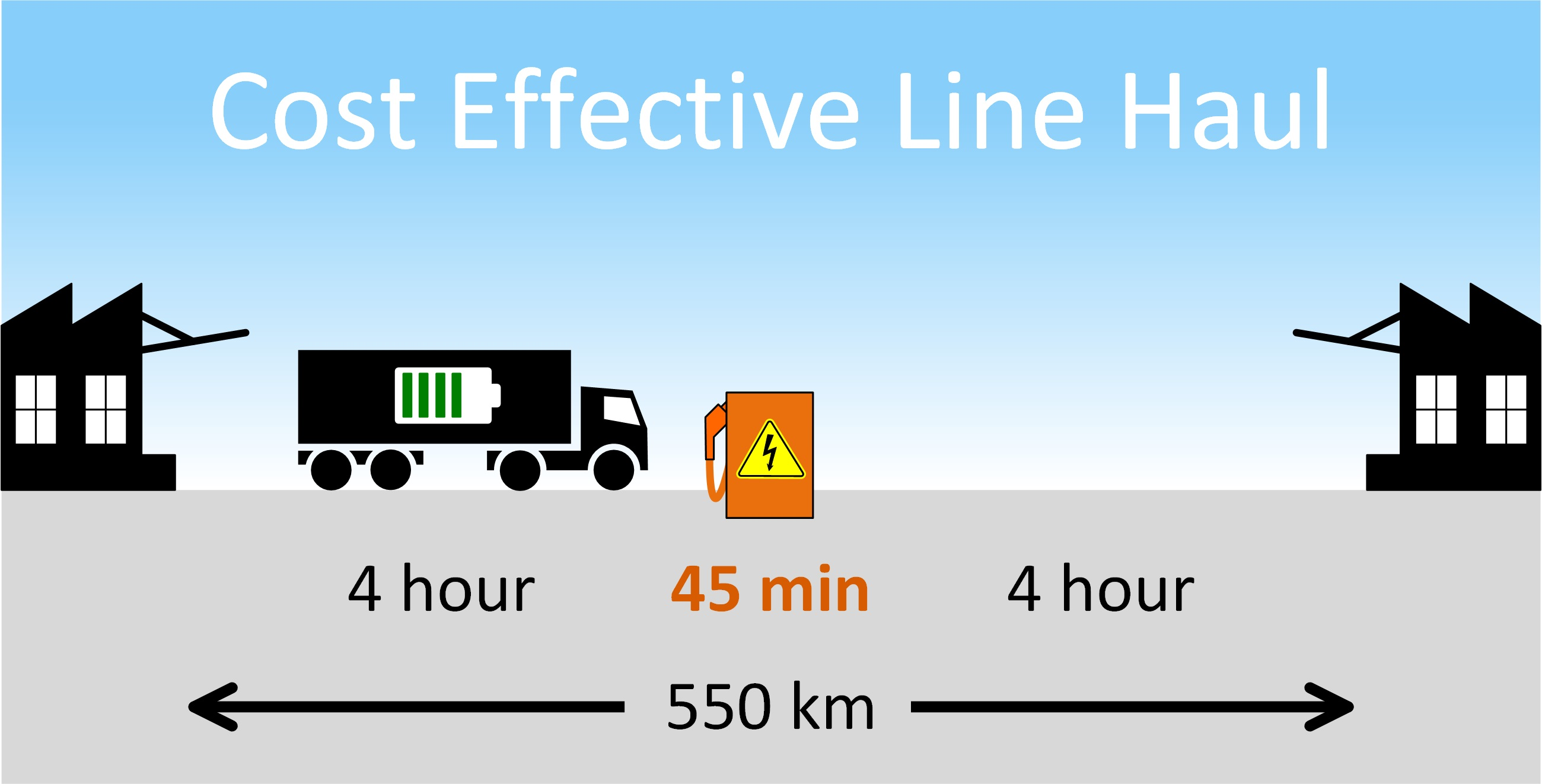
The company has two terminals, A and B, which are connected by a highway. Terminal A is located in Helsingborg on Sweden’s west coast and Terminal B is located in Stockholm, Sweden’s capital located on the east coast (see Figure 1). From the map, it is clear that this type of transport distance is sufficient to reach many cities in Europe from the closest harbour. Five times a week, the following procedure is repeated. Half of the trucks arrive at Terminal A and half arrive at Terminal B in the afternoon, following some local distribution tasks during the day. The trucks are then idle for a certain time, . At 6 PM, the first truck leaves the terminal and drives towards the other terminal. Thereafter, the other trucks leave the terminal one by one at a given interval, . Midway between the terminals, the drivers take a break, , at a rest area. This break is compulsory under the Driving and Resting time Rules and must be at least 45 min. After the break, the driver from Terminal A swaps trucks with the driver from Terminal B and the drivers then return to their original terminals. After arriving at their destination terminals, the trucks stand idle for a certain period of time, . Let the following values also apply: the distance between Terminals A and B—S; the mean speed of the trucks—; the trucks’ mean energy consumption per unit of distance travelled—; and the number of trucks leaving from each terminal—. For clarity, the charge losses are not explicitly modelled in this paper but their cost can be included in the price of electricity. The battery discharge losses and efficiency of the powertrain are also not explicitly modelled but are included in the trucks’ energy consumption. During the local distribution tasks that take place during the daytime, each truck has driven a distance, . This paper’s notation for the parameters and their values is listed in Table 1. In addition to driving each weekday during the year, each truck performs, on average, 50 extra night trips per year on the weekends. At the rest area, a charge-point operator has a public fast-charging station for trucks. So, in addition to the company’s private chargers at each terminal, the trucks can also be charged at the rest area using public fast chargers.
This paper investigates whether it is economical to use battery-electric trucks for the studied type of line haul and, if so, how the system should be designed. More specifically, this paper attempts to answer the following questions:
- What are the economic consequences for the company to change from diesel trucks to battery-electric ones?
- What power should the company’s private chargers have?
- What is the maximum extra cost of the reduced payload capacity due to heavy batteries?
- How many public fast chargers must be installed at the rest area by the charge-point operator and what should their power capacity be to meet the demand from the haulage company?
- Can the charge-point operator at the rest area expect a profit from the chargers if the stated company is their only user?
- Should a charge-point operator always meet the demands of its users? If not, how should the total power be selected?
3. Economic Consequences of Electrification for the Haulage Company
Many of the trucks’ main costs would remain approximately the same if the company replaced its diesel trucks with battery-electric ones. This includes the cost of maintenance and insurance, as well as the cost of the vehicle (excluding the battery in the case of electric trucks). Drivers’ salaries would also remain the same if charging took place during planned breaks. In addition, it is assumed that the second-hand value of the trucks would be comparable. The main differences would be the cost of diesel compared to the cost of electricity, as well as the cost of the battery, the grid connection, and the charger. In this paper, the costs are normalised and expressed in EUR per propulsion kilowatt-hour. The costs that would remain the same after the transition to battery-electric trucks are ignored since the company is interested in how the expenditure changes. In a recently published study [8], a cost function, , for the battery-electric truck is presented as follows:
where is the battery utilisation factor and is the charger utilisation factor. The cost parameters in the above equation are defined in Table 2. The parameter is the ratio of the energy from private charging to the total amount of energy that is consumed by the truck over its service life. The table shows the parameter values used in this paper. These values are the same as those used in a previous study [8]. The first term describes the cost of electricity when charging with a private charger; the second term gives the cost of public fast charging; the third term expresses the battery cost; and the last term gives the combined cost of the charger and grid connection. The battery utilisation factor is defined as the total energy consumed by the battery over its service life divided by the battery capacity. The battery utilisation factor uses the dimensionless unit, the equivalent full cycle (EFC). The charger utilisation factor is defined as the total energy delivered by the charger over its service life divided by the maximum energy that it can deliver over its service life. Thus, the charger utilisation factor is a dimensionless scalar from 0% to 100%.
The cost function expresses the cost of one truck with one private charger. However, even if the company has many trucks, the above expression can still be used, as it is assumed that there are as many private chargers as trucks. The battery-electric propulsion cost () should be compared to the diesel propulsion cost, , which is taken as 0.30 EUR/kWh, as in the above-mentioned study [8]. This corresponds to a diesel price of only 1.2 EUR/litre (excluding VAT) and a high power-train efficiency of 40%. The value of the diesel price is uncertain and most likely a bit too low, especially with the recent surge in diesel prices. However, it is possible that the current diesel price is only temporary. Furthermore, it is necessary to ensure that the reference value for diesel is not too high. If electric trucks can be shown to be competitive at the stated diesel price, then there is more certainty about this paper’s conclusions. To calculate the cost function value, it is necessary to find the values of and the utilisation factors. These parameters depend on the charging strategy, as shown below.
This case study assumes that the vehicle will have the same energy consumption throughout its service life. This allows the battery to be sized solely for this specific type of use. Due to battery ageing and safety margins, it is assumed that only a share of the battery capacity will be used. Let this share be and the useful capacity . This can be expressed as:
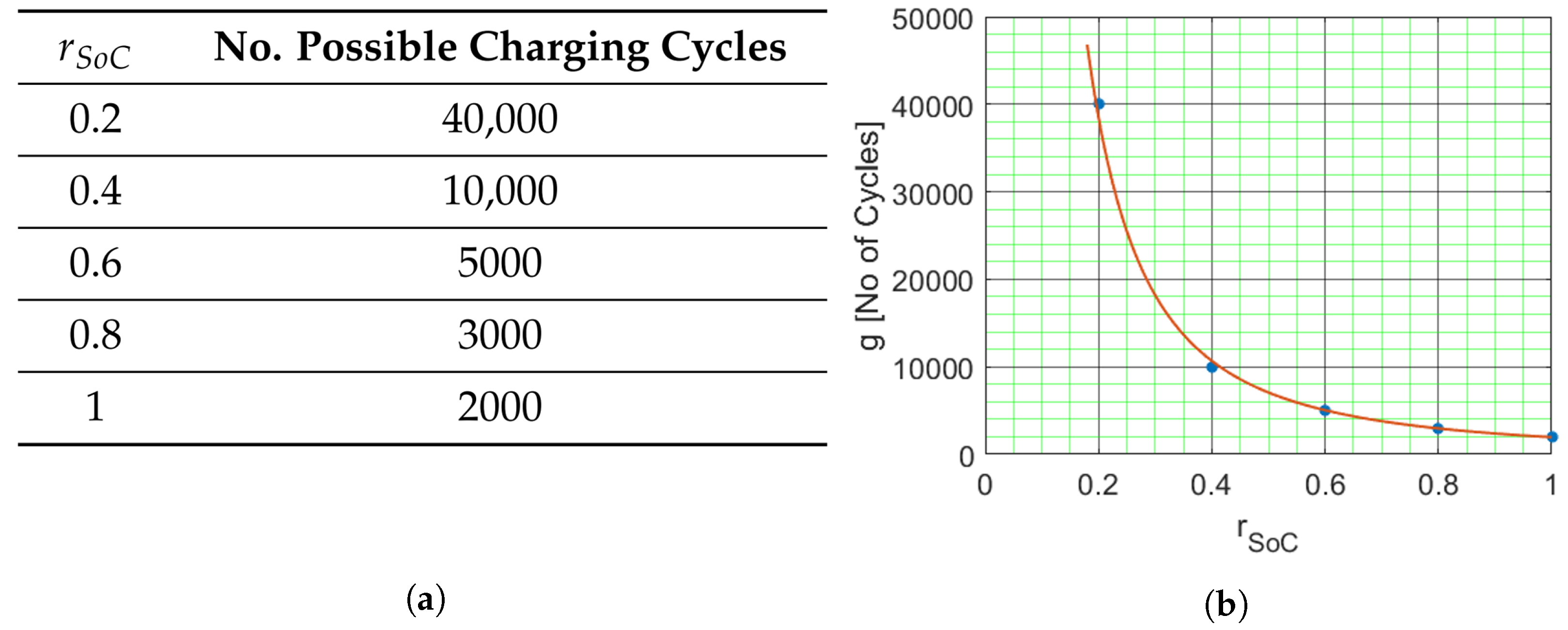
where is the battery capacity. The number of possible charging cycles for a modern lithium battery is assumed to depend on according to the table in Figure 2a. The exact number of lifetime cycles varies for different types of Li-ion cells but the general trends are the same, that is, the number of cycles increases faster than the decrease in cycle depth, resulting in a total life–energy throughput. This can be seen in studies such as [20]. The numbers used here are selected based on the tests and data sheets for several different Li-ion cells. The cycle life of the battery depends on many factors, for example, the temperature. It is assumed that the battery management system will keep the temperature in the allowed temperature range.
So, how many cycles are needed during the battery’s service life? The battery must be able to cover the distance without being charged. However, if the battery is too heavy, there is a risk of losing payload capacity. Therefore, a company’s primary aim is to size the battery so that it just can handle the distance without charging. This means that the entire useful capacity must be charged at a rest area each day the truck is operating. Thus, each truck performs three charging cycles each weekday for seven years (the lifetime value of the battery according to Table 2), plus two extra charging cycles on the weekends 50 times per year. Thus, the number of charging cycles in the battery’s service life, , can be determined as follows:
Since the value did not match the table values in Figure 2a, a power function is fitted to the table values with the result and (see the red curve in Figure 2b). By solving the equation , we obtain the root:
The required useful battery capacity is given by:
This results in a battery capacity of:
The battery utilisation factor can now be calculated:
which is a high value and results in a low battery cost. The reason for this high value is that the truck is driven in two shifts and often performs three charge and discharge cycles per day.
Since the price of the chargers and grid increases with the charger power, , private chargers should be as low-powered as possible. However, the charger must still be able to charge the useful capacity in the time and and, therefore:
In real life, there may be reasons to oversize the chargers slightly but this is not discussed here. From the definition of the charger utilisation factor, one obtains
where is the total amount of energy delivered by the private charger over its service life. For the weekdays, the private charger must deliver enough energy for two cycles each day. For each of the weekend trips, the private charger must deliver enough energy for one cycle. This is because the battery’s entire useful capacity will be charged at the rest area each day the truck is operating. Each cycle demands energy of kWh. Thus, the energy delivered by the private charger is given by:
which gives:
So far, the utilisation factors for the private chargers and batteries have been determined. It is now necessary to determine the value of to find the cost of battery-electric propulsion using Equation (1). Over its service life, a truck performs one day trip and one night trip every weekday for seven years. So, each weekday involves charging the entire useful capacity three times. The truck also performs 50 extra night trips per year, with each night trip resulting in the entire useful battery capacity being charged twice. Thus, the total energy consumed over a truck’s service life is given as:
Since is the energy charged using a private charger divided by the total energy consumed over the truck’s service life, the result is:
Using this value, the values for the utilisation factors, and the values from Table 2 in Equation (1), the following cost-function value is obtained:
By evaluating each term in Equation (1), the price of energy from private charging is 0.05 EUR/kWh, the price for public fast charging is 0.14 EUR/kWh, the battery price is 0.06 EUR/kWh, and the price of the private charger and grid is 0.07 EUR/kWh. Notice that these individual costs are now normalised per the total energy consumption and not the amount of energy from the respective chargers themselves. This means that fast charging that costs 0.4 EUR/kWh will cost 0.14 EUR/total kWh since only 35% of the total energy comes from fast charging.
Thus, these particular electric trucks have proven to be slightly more expensive than diesel trucks. The savings will be negative and the annual value is:
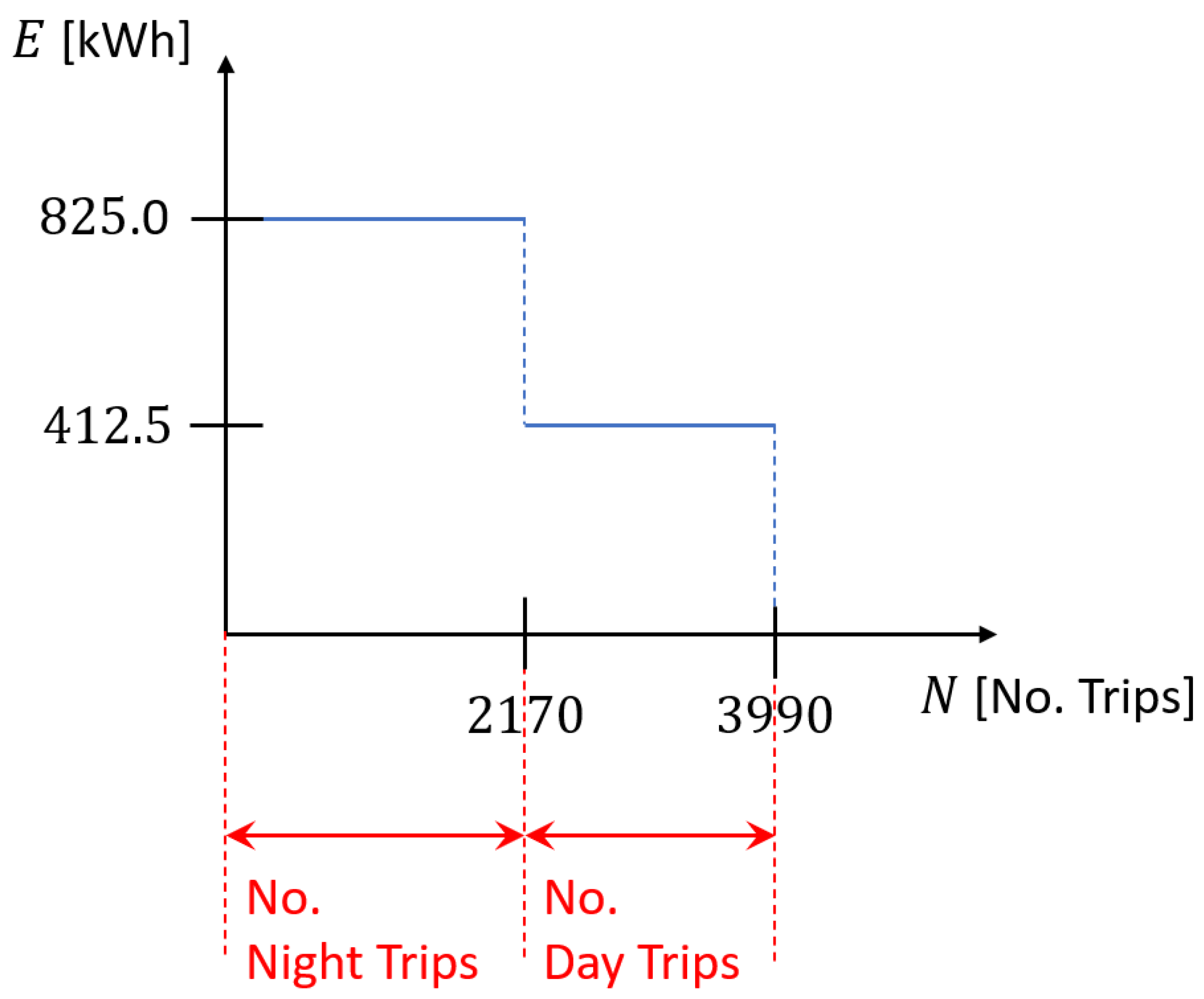
Since the above calculations indicate extra costs for the company, a more cost-efficient charging strategy should be used. In considering the above individual costs, it becomes apparent that the cost of public fast charging is by far the greatest. Is it possible to reduce this cost? Yes, if the trucks have batteries large enough to handle long night trips with less reliance on public fast charging. Even so, this will increase other costs such as the cost of a large battery. If all the day trips are viewed as one type of trip consuming energy and all the night trips as another type of trip consuming energy , the energy consumption for the trips can be presented in an energy distribution diagram, similar to that introduced in [8]. There are five daytime trips each week for seven years, resulting in 1820 day trips in a truck’s service life and equally as many night trips during the week. However, an additional 50 night trips per year equates to 2170 night trips in a truck’s service life. The energy distribution diagram for each truck is shown in Figure 3 and it is a “two-step rectangular” type [8].
It was shown in [8] that for a two-step rectangular energy distribution diagram, the lowest cost-function value is obtained either when the battery can handle the energy needs for the low-energy-consumption trips or when the battery is sufficiently large to handle the complete energy needs of all trips without being charged. A certain level of care must be exercised since the prerequisites of that analysis are not in complete agreement with those of this study. Nevertheless, the special case of a battery that can handle high-consumption trips still warrants investigation.
For a large battery, the useful capacity must be able to handle an entire night trip without charging. Thus,
The power of the charger must be considered, as it needs to meet the charging demand for a battery’s entire useful capacity in time and half that capacity in time . Again, this yields a charger power of:
So, what value is reasonable for ? As seen in the energy distribution diagram in Figure 3, the battery must now perform 3990 cycles during its service life. Furthermore, 1820 of these will be half cycles. Thus, may be set so that the battery can survive 3990 major cycles. This also gives an even better safety margin compared to the small battery. By solving the equation , the following root is obtained:
This results in a battery capacity of:
The battery utilisation factor is given by the total energy consumed by a truck over its service life divided by the battery capacity. The total energy consumed is obtained from the area under the curve in the energy distribution diagram in Figure 3. Thus,
As expected, a lower value for the battery utilisation factor is obtained compared to a small battery. The result is a rising battery cost. The charger utilisation factor is defined as follows:
In this case, is all the energy consumed by the truck in its service life, as all the energy comes from a private charger. This also implies that . The charger utilisation factor increases compared to a small battery. This is reasonable since the chargers (which have the same power) deliver more energy over their service life. By inserting the values of the utilisation factors and the values from Table 2 into Equation (1), we obtain:
The largest cost is that of the battery, 0.10 EUR/kWh, followed by the cost of the energy from the private charger, 0.08 EUR/kWh; the cost of the private charger and grid, 0.07 EUR/kWh; and the cost of public fast charging 0 EUR/kWh. Due to rounding, the individual cost appears to total more than the overall cost. This charging strategy appears promising and the company’s savings can now be calculated:
where is the total energy consumed by one truck over its service life. This is obtained from the area under the curve in the energy distribution diagram.
Firstly, the calculations show that under these circumstances, battery-electric trucks are competitive compared to diesel trucks. Secondly, it shows that the choice of battery capacity could have a major impact on the cost effectiveness of battery-electric trucks. Although the cost of the battery is large, the overall cost of ownership may be lowered by selecting a large battery, as the price of public fast charging may also be high. The trade-off between battery size and the share of public fast charging may be fairly simple to handle if the price picture and charging opportunities are known. However, there are more trade-offs to consider such as the trade-off between reduced costs and any losses in payload capacity. The potential cost of losing payload capacity is estimated in the next section.
4. Cost of Losing Payload Capacity
Since the calculations indicate that a large battery is cost effective, this section aims to estimate the cost of losing payload capacity. Note that the maximum extra cost calculated below is only valid if the trucks always carry the maximum weight. However, for most trucks, this is not the case. Even with large batteries, there are seldom any extra costs. It is often the volume of the truck that limits the payload and the truck may not even be full.
For batteries weighing up to 1.5 tonnes, it is assumed that there is no loss in payload capacity, whereas for heavier batteries, the loss of payload capacity equals the weight of the battery minus 1.5 tonnes (see Appendix A for more details). For increased readability and generality, let tonnes. The total cost of operation, , for a truck weighing 40 tonnes is about 0.9 EUR/kWh (see Appendix B for more details) and it has a payload capacity, , of 27 tonnes (see Appendix A). The battery capacity per ton, , is 170 kWh/tonne (see Appendix C), which leads to a reduced payload capacity, , of
The reduction in the maximum payload is 3.0 tonnes for a small battery and 5.6 tonnes for a big battery. The new payload capacity, , is given by
The ratio of the new required number of trucks to the number of trucks when there was no loss of payload capacity, , can now be expressed as
Finally, the maximum extra cost of losing payload capacity, , becomes
and with the values for the small and large batteries, one obtains
and
Due to this potentially high indirect cost of large batteries, the company would likely prefer the small battery solution, provided that the price of public fast charging is low enough. Thus, the cost of a reduced payload will be high if the goods being transported are high-density items such as stone slabs. Equally, it might as well be zero if the goods being transported are low-density items such as bundles of tulips. Therefore, it can be concluded that due solely to the payload density, battery sizing may sometimes vary among trucks being driven on identical routes.
5. Number of Chargers and Price of Charging at the Fast Charging Station
The above calculations suggest that the haulage company would want its batteries to be sized to eliminate the need for public fast charging if the price of public fast charging is 0.4 EUR/kWh. Thus, it would be interesting to investigate whether the charge-point operator planning to install chargers in the rest area could lower their prices. The charger owner’s costs comprise the costs of the electricity, chargers, and grid connection. As mentioned earlier, the costs of the charger and the grid are assumed to be proportional to the charge power and cost per kWh, , and can be expressed as
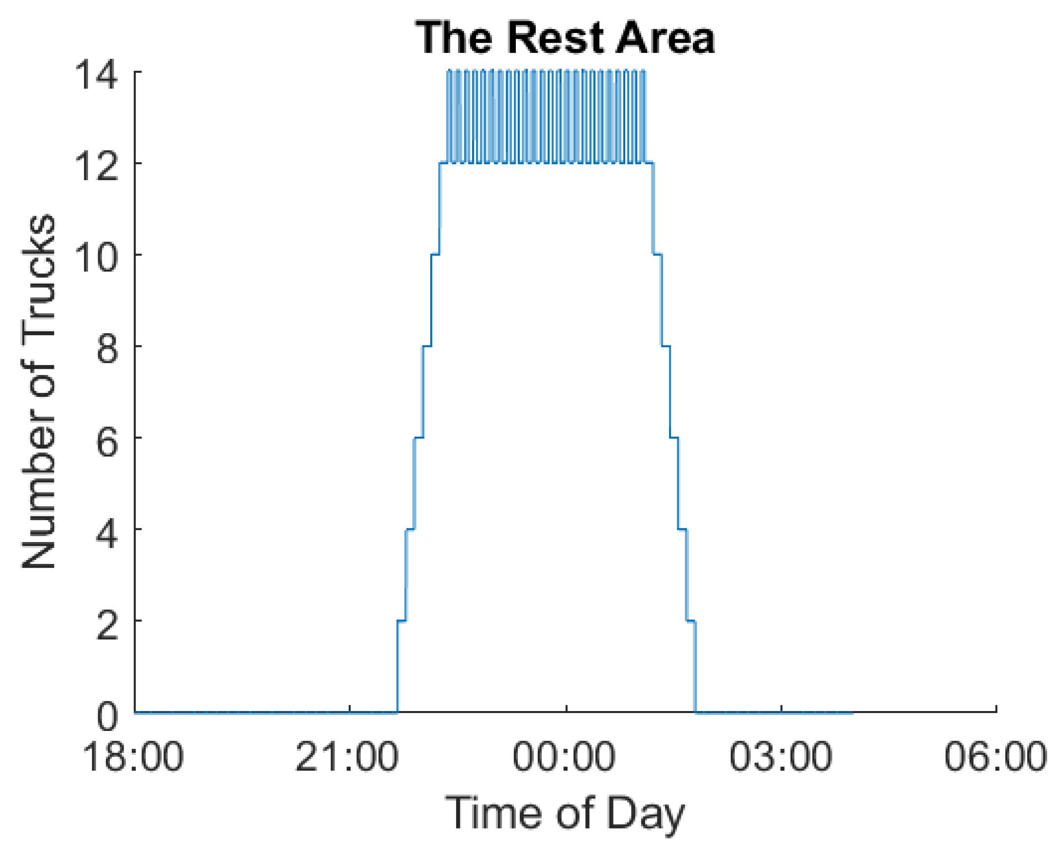
Firstly, one may assume that the haulage company would fully charge its trucks at the rest area. The drivers have a 45-min break and this is the time each truck has for charging. So, how many chargers would be needed? Thirty trucks depart from each terminal at intervals of min, as the terminal and gate personnel do not have the capacity to send them off simultaneously. If the first two trucks leave Terminals A and B at 6 PM and then drive the km to the rest area at a mean speed of 75 km/h and charge for 45 min upon arrival, the number of charging trucks (as a function of time) can be determined through simulations. The results are presented in Figure 4.
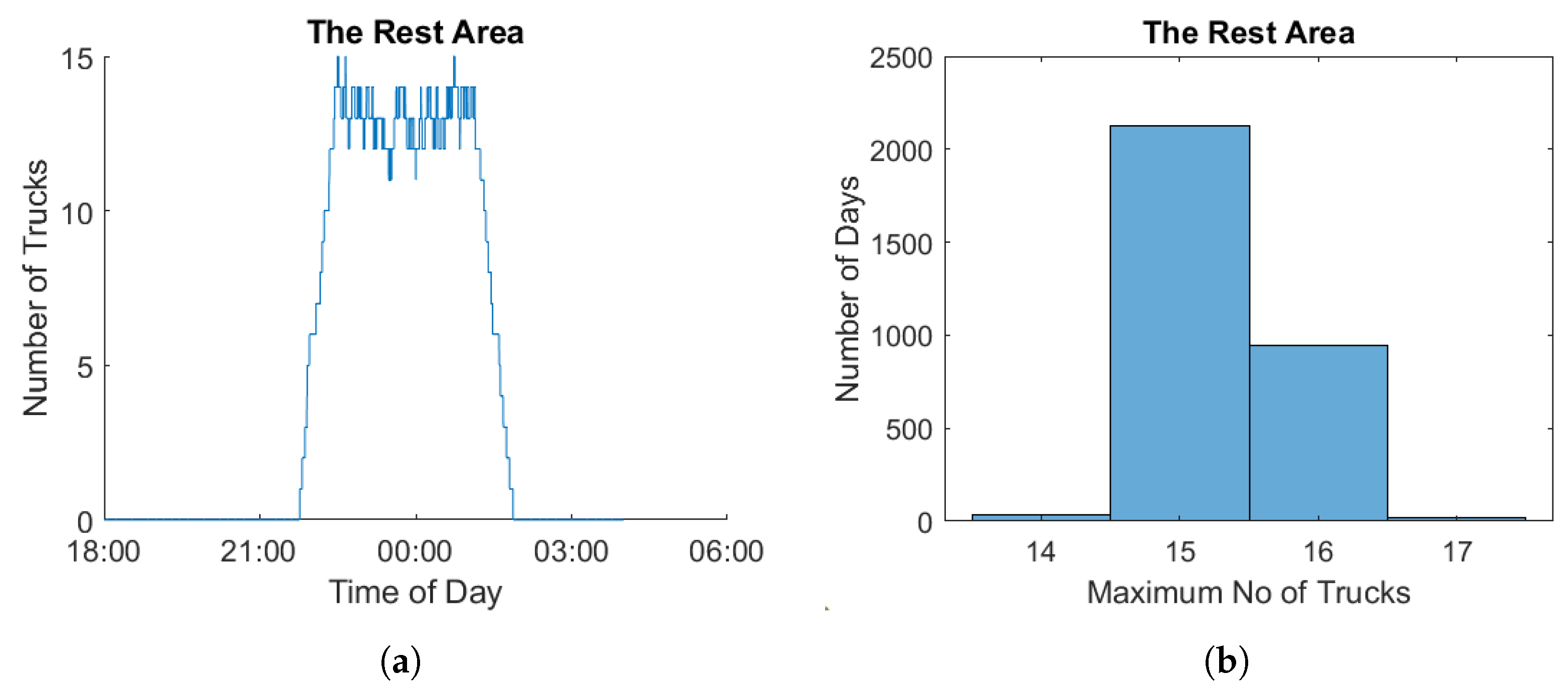
When considering Figure 4, it may appear that 14 chargers would be sufficient. However, the results demand perfect timing with no delays. Therefore, it would be interesting to see what would happen if the trucks were delayed. The company claims that delays over 15 min are very rare. Thus, a new simulation was run in which it was possible to delay the trucks. For each truck, the delay was set as the magnitude of a random number drawn from a normal distribution with the expected value of zero minutes and a standard deviation of five minutes. Figure 5a shows the number of trucks charging for one night at the rest area as a function of time when the trucks are delayed. As seen in Figure 5a, the maximum number of chargers needed on this day was 15. It appears that the delay can increase the number of chargers needed to avoid queuing and further delays. Figure 5b shows a histogram in which the x-axis value represents the maximum number of chargers needed on one day and the height of the bar represents the number of such days that occur in a 10-year period (the trucks operate almost six nights per week). As seen in the histogram, for the selected model and parameter settings, 16 chargers are needed at the rest area. The fact that there is sometimes a demand for 17 chargers is not considered a problem, as this only happens twice a year. The results do not change significantly when the standard deviation is changed by ±2 min.
The conclusion is that the number of chargers, , that should be installed at the rest area is
Each charger must be able to charge a truck’s entire useful capacity in time . Thus,
Since the trucks charge their entire useful capacity five times per week for seven years, with 50 extra charges per year on the weekends, the chargers will deliver the following energy over their service life:
and the charger utilisation factor becomes
So, if the charge-point operator has no customers other than the haulage company being studied, the cost of the chargers, according to Equation (30), will be
It seems possible to lower the price from the originally intended 0.4 EUR/kWh. So, how low must the price be for the haulage company to consider using small batteries and fast charging for their entire useful capacity at a rest area? The company would probably select the smaller battery if it can achieve an equally low cost as large batteries, as increasing the payload capacity also offers gains. Thus, the required fast-charging price may be determined by solving the equation:
using the values for the small batteries, as follows:
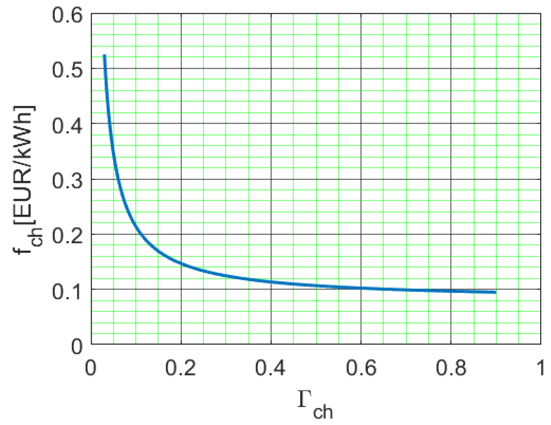
Initially, this seems hard to achieve, as this value is below cost when the studied haulage company is the only user, as determined by Equation (35). However, as seen from Equation (30), the normalised cost to the charge-point operator strongly depends on the charger utilisation factor. Figure 6 shows as a function of .
In Figure 6, it can be seen that the value of drops quickly for low and increasing values of the charger utilisation factor. Thus, it might be possible to have both profitable charging stations and cheap fast charging if the utilisation factor is sufficiently large. Based on the figure, it seems that roughly 20% or more should be considered “large”. The figure shows that is a little below 0.17 EUR/kWh for higher charger utilisation factors. The treated haulage company occupies the chargers for less than four hours, which corresponds to 17% of the day. Since brief investigations from the available data [21] of the road midway between Helsingborg and Stockholm indicates that the traffic flow of heavy vehicles with trailers is quite even over the day, it should be possible to find other haulage companies with complementary driving patterns to the studied one. Consequently, it seems very likely that at least the same level of use of the chargers is possible by other companies during the remaining 83% of the day. Thus, we claim that the charger utilisation could be at least 20%, and Equation (30) then yields a cost of EUR/kWh. This could be low enough to be profitable. If, for example, a charger utilisation of 25% is reached, it would lead to EUR/kWh, at which point the chargers appear profitable. However, even if we think it is realistic to reach a charger utilisation of at least 20%, it is important to clarify that the following paragraph relies on the assumption that the public chargers could reach a utilisation rate of at least 20%.
So, if the public fast chargers are utilised sufficiently, the haulage company will have a normalised cost for battery electric propulsion of 0.24 EUR/kWh, of which the cost for private charging is 0.05 EUR/kWh, the cost of the public fast charging is 0.06 EUR/kWh, the cost of the battery is 0.06 EUR/kWh, and the cost of the charger and grid is 0.07 EUR/kWh. The indirect cost of any loss of payload capacity would likely be low. The calculations presented in this paper strongly indicate that electric trucks would be more cost efficient than diesel trucks for haulage companies that have similar driving patterns to the company studied here and do not regularly carry heavy goods. Note that this might not be the case for haulage companies with driving patterns that deviate significantly from those in this paper, as the cost effectiveness of battery-electric trucks is heavily dependent on driving patterns [8]. However, the method presented in this paper can be used to evaluate the economic consequences for haulage companies that use other driving patterns. A more detailed description of the selection of a cost-effective battery size for different energy distribution diagrams was presented in [8].
If, however, the charge-point operator cannot offer public fast charging at a sufficiently low price due to problems related to reaching a high charger utilisation, the haulage company should go with the large battery, even if this scenario seems unlikely to the authors. In the worst-case scenario, when fast charging is expensive and the company regularly carries heavy goods, diesel trucks might be the most cost effective out of the analysed solutions.
It is also worth mentioning that since the studied haulage company uses almost 10% of the chargers’ capacity, it may want to consider buying its own fast chargers and then selling charging services to others when the chargers are idle.
6. Selecting Total Power for a Fast-Charging Station
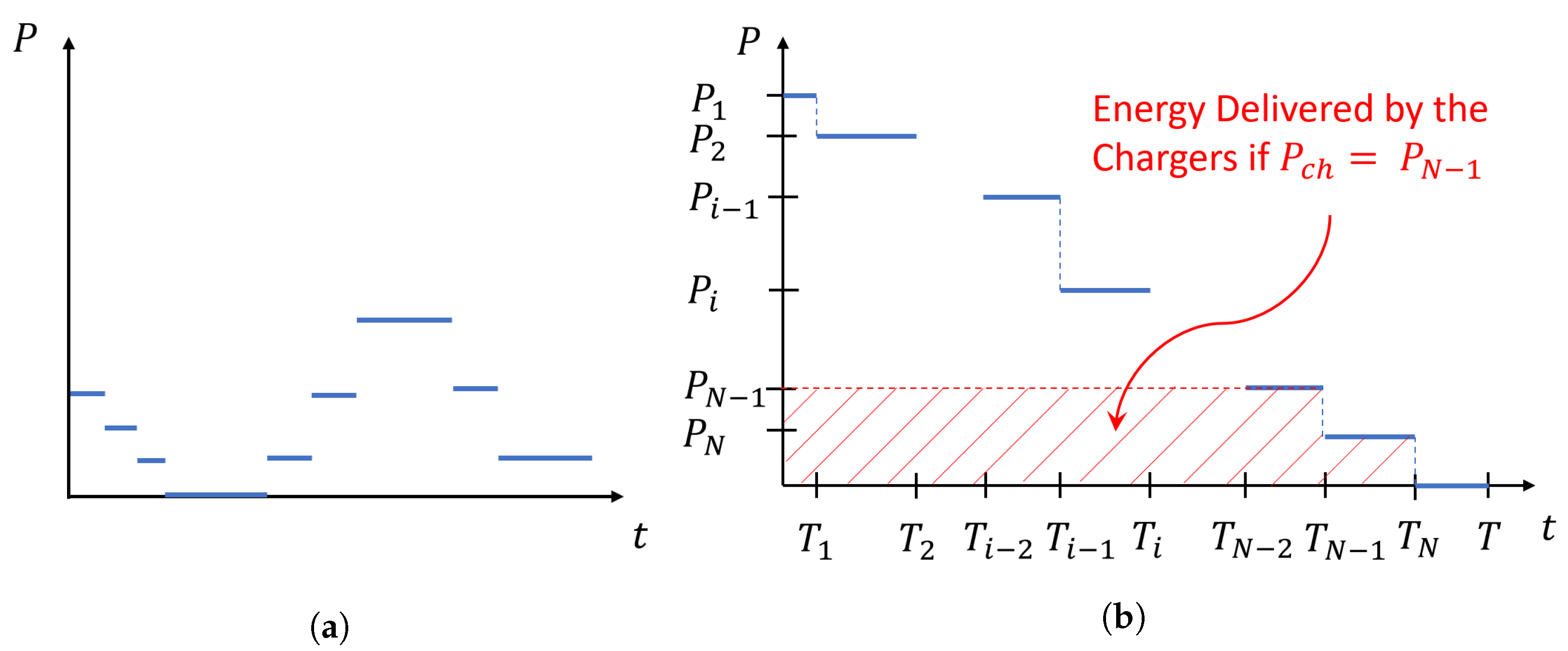
The previous section showed that to meet the demands of the haulage company, 16 chargers should be installed in the rest area. Fully meeting this demand is probably a given. The haulage company would be a key customer and charge a large amount of energy six days a week. However, the demand, for example, at lunchtime would likely be quite high, as many drivers probably have a scheduled break at that time. It then becomes a matter of whether it is cost effective to meet the peak demand for charging. If not, how much of the peak demand should be met? To investigate this, it was assumed that the time-variable demand for public fast charging could be estimated for a given fixed price level. In other words, the selected price does not vary over time. Since there is a discrete number of trucks needing to charge, it is natural to assume that the power demand for charging will be a step function of time, as in Figure 7a. If the power demand is arranged by magnitude over the service life of the chargers, the result is a diagram that we call the power demand distribution (see Figure 7b), where represents the power demands of different durations according to the figure and . On the right-hand side of the figure, the red, striped area represents the energy that would be delivered by the chargers over their service lives for the selection .
The power demand, , can be expressed as
where is the total duration in which there is a demand to use at least one charger. Thus, the notation is introduced.
To choose the total power of the charging station wisely, the profit, I, for the charge-point operator is now expressed as follows:
Note, that in this context, is the total energy delivered by the charging station over the service life of the chargers, is the total power of the charging station, and T is the service life of the chargers. In the above equation, the first term on the right-hand side is the total income of users over time T, the second term is the total cost of the electricity over time T, and the last term is the total cost of the chargers and the grid connection over time T. Let
and Equation (39) becomes
The charge-point operator can directly affect two of the parameters in Equation (41), namely by setting the price for public fast charging and by determining the total power of the chargers when investing in them. These choices will indirectly affect the total energy delivered by the chargers, . This is because the price for public fast charging will affect demand and the total power of the chargers will limit their capacity to deliver energy. Now, we investigate when the chargers are profitable and how to select their total power (number of chargers) and thus maximise the profits for the charge-point operator. Assume that a given fixed price level has resulted in a power demand distribution. From this distribution, the aim is to find the total power of the charging station, , to maximise the profits for the charge-point operator. Since the charge-point operator selects the number of chargers, it may be assumed that , where . The case when corresponds to there being no chargers at all, whereas corresponds to the peak charging demand being met.
The energy delivered by the chargers over their service life is now limited by the values of and . Thus, it is now clear that depends on n according to
which can be compared to the right-hand side of Figure 7b, with . Now, can be inserted into Equation (41) to determine the profits, giving
An adequate criterion for a profitable charger station is
which means that
Since , and , we can write
If the above inequality is satisfied, the chargers will be profitable when . If the inequality is satisfied, how can the chargers be even more profitable when ? To investigate this, let us assume that the chargers are profitable for . Will the profits I then be larger if is used? The answer is yes, if, and only if, the increase in the first term is larger than the increase in the second term in Equation (41). Thus, the profits when increase compared to the profits when if, and only if,
Since , this is equivalent to
However, if the inequality is not satisfied, the income will decrease if is allowed to assume even higher values than , for example, , where , since the same procedure would lead to increased profits when compared to the profits when if, and only if,
As before, since , this is equivalent to
However, since the inequality Equation (48) was not satisfied, will this one will also not be satisfied, as . Thus, the above calculations and mathematical induction allow us to conclude that
and to maximise the profits for the charge-point operator (and assuming the chargers are profitable), the charger power should be chosen such that
where k is the smallest integer in the set that fulfils the inequality. It appears that the power of the chargers would only meet the full demand if the highest power is used for a sufficiently long time. With the different values used in this paper, the peak demand must last for 4% of the service life of the chargers if the price of public fast charging is 0.4 EUR/kWh or 15% if the price is 0.17 EUR/kWh. It is worth mentioning that the sole aim of this calculation is to maximise the profits for a given power demand distribution when public fast-charging prices are fixed. However, it does not consider effects such as losing a customer to a competitor with more chargers available or the loss of all charging undertaken by that customer, not just the peak-time charging.
7. Discussion
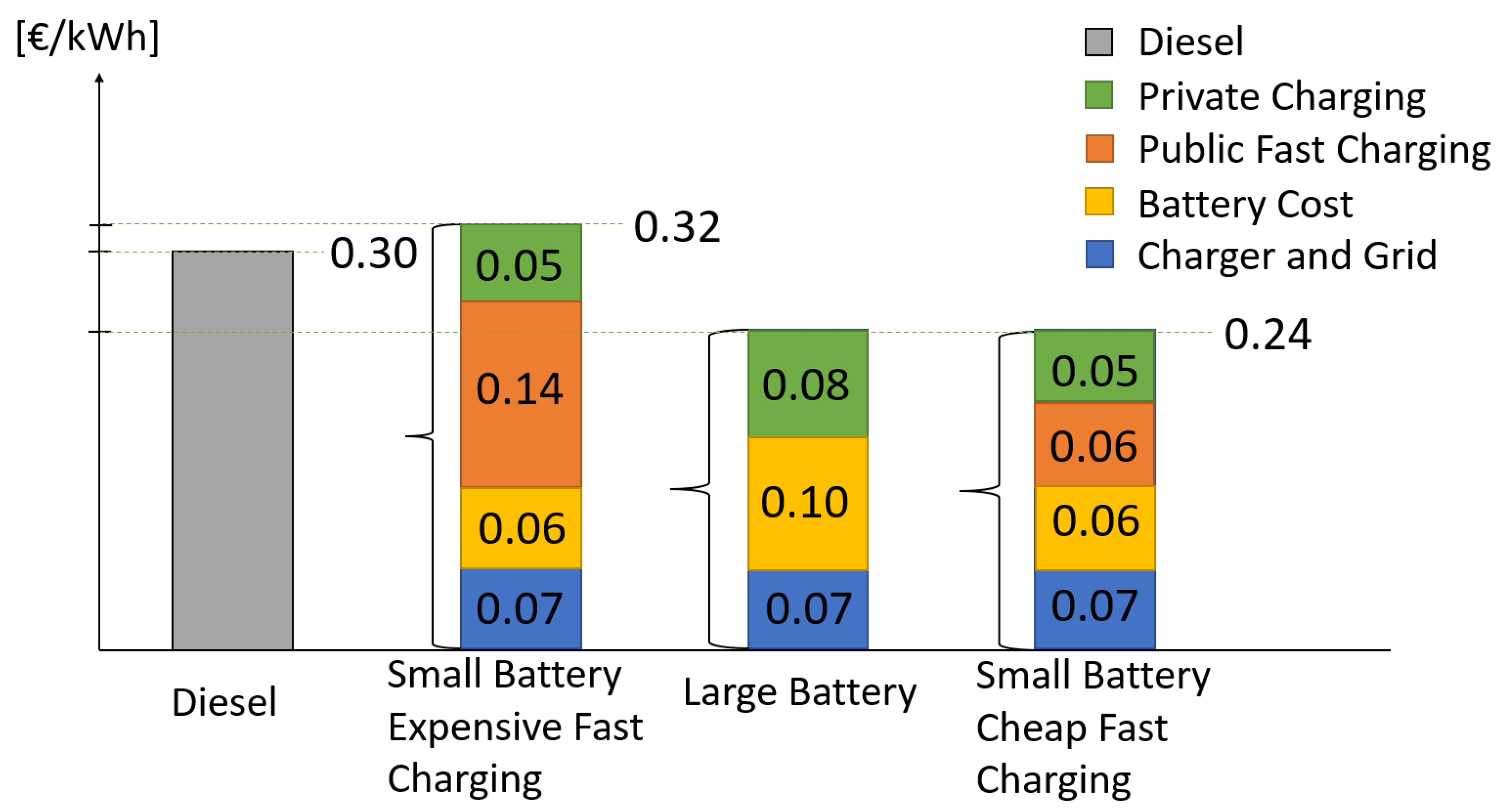
This paper shows that long-haul battery-electric trucks can compete with diesel trucks, even if the price of diesel fuel is only 1.2 EUR/litre (excluding VAT), and even more so if the price of diesel fuel stays at the current high level of 1.8 EUR/litre. However, what makes the problem complex is the difficulty of determining the battery capacity and charging strategy if there is significant price uncertainty in public fast charging. At the same time, it is hard to set public fast-charging prices without knowing how much the chargers will be used. Additionally, the investment made by one party can be risky if the other party changes its strategy. For example, if a haulier starts buying larger batteries, the need for public fast charging may greatly diminish, which is bad for the charge-point operator. Similarly, if the haulier has chosen small batteries, a price rise in public fast charging will be problematic. However, what benefits the transition from diesel trucks to battery-electric trucks is that these problems will likely decrease over time. This is because charging in the long run will be a very competitive business with few entry barriers. However, during a rapid transition, the competition may be weaker since there are some additional entry barriers such as high investment risks during a turbulent industry transition, a temporary lack of available grid capacity, and long installation waiting times. However, the more common battery electric trucks and vehicles become, the easier it will be to achieve high charger utilisation factors and thus lower public fast-charging prices. Furthermore, the price picture will probably change in favour of battery-electric trucks due to increased production volumes and technological advancements. Figure 8 compares the costs of the main alternatives for the studied haulage company. In the figure, all the values are in EUR/kWh and the bar height represents the total cost of a given strategy. The indirect cost of a reduced payload is not included, as this depends on the type of goods being transported. This can vary from zero to the values estimated in this paper. (The individual costs of the battery-electric truck with a large battery seem to add up to more than the total cost, but this is due to rounding.) As stated earlier, the haulier is likely to select the strategy represented by the fourth bar. Provided a low price for fast charging can be secured, this will make the cost of propulsion energy lower than the cost of current diesel trucks. Additionally, there will be less of a reduction in the payload capacity compared to the large battery strategy.
In the previous section, the price of electricity and public fast charging was assumed to be fixed. However, is it likely that a charge-point operator will have a fixed price for their users? Maybe not. In reality, the demand for charging power will vary over time, which can be demonstrated using a demand power distribution such as the one in Figure 9a. This illustrates that for , there is a much greater demand than the charging station can supply. This means that the charge-point operator has an opportunity to increase the price of public fast charging and still sells the same amount of energy but increases the profits. It may also be possible to move users from rush hour to other times by setting a higher price during rush hour and a lower price at other times (see Figure 9a,b). The mean value of the difference in price for public fast charging and electricity may even be the same but, due to the increase in , the profits will still increase. Again, consider Figure 9 as an example. It may be argued that time-variable pricing will also benefit users, as it allows fast charging to be offered exactly when it is needed by those who really need it and can pay for it. It also means that users who move to other charging times will be rewarded with lower prices. How to select a price for public fast charging is a very complex question and requires a thorough investigation of its own. It is not possible to predict charging prices based on this brief analysis. Still, this analysis shows that a low price seems achievable. It also highlights the many ways in which pricing and the haulier’s charging strategy can be changed to increase charger utilisation and facilitate even lower prices.
8. Conclusions
Based on the above analysis, the following conclusions can be drawn for the type of long-haul trucks studied in this paper.
- Battery-electric trucks with driving patterns similar to those of the haulage company studied in this paper appear to be more cost effective than today’s diesel trucks, at least if they do not regularly carry heavy goods. One reason for the competitiveness of electric line-haul trucks is that they have a high level of battery utilisation and can be charged during mandatory breaks.
- The study indicates that the main uncertainty factors (in terms of knowing what charging strategy to use) are the price of public charging and the density of the goods.
- The choice of battery capacity is strongly influenced by the price of public fast charging. For the case studied in this paper, the price of fast charging has to be 0.17 EUR/kWh if the haulier chooses the small battery rather than the large one. The size of the battery could have a significant impact on the total cost of ownership.
- The cost per kWh for public fast charging drops significantly as charger utilisation increases. A charger utilisation factor of approximately 20–25% should be sufficient to offer fast charging at a low price such as 0.17 EUR/kWh.
- The ratio is an important parameter when analysing the profits of a charge-point operator, where is the combined cost parameter of the charger and grid and is the difference between the price of public fast charging and the price of electricity. This is intuitive since the profits increase with but decrease with . With the values used in this paper, the ratio ranges from 4 to 15%. This range is caused by the price uncertainty of public fast charging.
- For public fast charging at fixed prices, a charge-point operator can only be profitable if, and only if, the demand for charging (expressed as a share of the service life of the chargers) exceeds .
- For public fast charging at fixed prices, the charge-point operator cannot meet the peak demand for charging in order to maximise profits. The only exception to this is when the share of the peak-time demand equals at least of the service life of the chargers.
- If the chargers can be profitable for a given demand power distribution, the profits of the charge-point operator (at a fixed price) can be maximised according to the procedure described in Section 6.
9. Future Work
This paper shows that cheap public fast charging is possible if the charger utilisation is high. Naturally, a high level of charger utilisation can lead to extensive problems with queuing at charger stations. Thus, an important question for future research is whether high levels of charger utilisation can be achieved while also having high levels of charger availability at fast-charging stations.
This paper also shows that the indirect cost of a reduced payload can vary from zero to very high values. This indicates that different types of transport on the same route can select different charging strategies or favour, for example, hydrogen fuel-cell powertrains. It will be crucial to investigate which types of transport are likely to use the different solutions.
Author Contributions
Conceptualisation, J.K. and A.G.; methodology, J.K.; software, J.K.; formal analysis, J.K.; investigation, J.K.; writing—original draft preparation, J.K.; writing—review and editing, J.K. and A.G.; supervision, A.G. All authors have read and agreed to the published version of the manuscript.
Funding
This research was funded by the Swedish Transport Administration, TripleF, grant number 2020.3.2.32.
Data Availability Statement
Not applicable.
Acknowledgments
Financial support from the Swedish Transport Administration has been gratefully received.
Conflicts of Interest
The authors declare no conflict of interest. The funders had no role in the design of the study; in the collection, analyses, or interpretation of data; in the writing of the manuscript; or in the decision to publish the results.
Abbreviations
The following abbreviations were used in this manuscript:
| BEV | Battery-electric vehicle |
| EFC | Equivalent full cycle |
Nomenclature
| Battery capacity (kWh) | |
| Battery capacity per tonne (kWh/ton) | |
| Useful battery capacity (kWh) | |
| Battery cost (EUR/kWh) | |
| Combined price for charger and grid (EUR/kW/year) | |
| Diesel cost (EUR/kWh) | |
| Difference in price between public fast charging and electricity (EUR/kWh) | |
| Cost of driving a 40-tonne truck (EUR/kWh) | |
| Electricity cost, private charging (EUR/kWh) | |
| Electricity cost, public fast charging (EUR/kWh) | |
| The maximum extra cost of losing payload capacity (EUR/kWh) | |
| The trucks’ energy consumption (kWh/km) | |
| The total energy delivered over the service life of the chargers (kWh) | |
| Total propulsion energy consumed over a truck’s service life (kWh) | |
| Cost function for the trucks (EUR/kWh) | |
| Cost function for the fast chargers (EUR/kWh) | |
| Number of possible charging cycles for the battery (—) | |
| Battery utilisation factor (equivalent full cycles) | |
| Charger utilisation factor (—) | |
| I | The profit for the charge-point operator over time T (EUR) |
| Battery weight limit for loss of payload (tonne) |
| New payload capacity (tonne) | |
| Payload capacity for a 40-tonne truck (tonne) | |
| Reduced payload capacity (tonne) | |
| Number of charging cycles in the battery’s service life (—) | |
| Number of chargers in the rest area (—) | |
| Number of trucks leaving from each terminal (—) | |
| Charger power (kW) | |
| Demand power (kW) | |
| Ratio of private charging to the total amount of energy (—) | |
| Share of battery capacity that could be used (—) | |
| Ratio of the number of new trucks to the number when there was | |
| no loss of payload capacity (—) | |
| S | Distance between terminals (km) |
| T | Service life of truck, charger, and battery (year) |
| Idle time for the trucks in the afternoon (hours) | |
| Idle time for the trucks in the morning (hours) | |
| Duration of the drivers’ breaks (minutes) | |
| Annual driving time for the trucks (hours) | |
| Time interval between trucks (minutes) | |
| Time when there is demand for at least one charge (years) | |
| Mean speed of the trucks (km/h) |
Appendix A
This appendix estimates the payload of a diesel semi-truck and then estimates the weight difference between an electric and a diesel truck to find out how much the maximum payload is reduced by the battery weight.
A conventional diesel 4 × 2 tractor weighs about 6.5 tonnes [22] and an empty semi-trailer also weighs 6.5 tonnes [23]. Since the maximum gross weight is 40 tonnes, the diesel semi-truck can have a maximum payload of 27 tonnes.
The weight difference between a diesel powertrain and an electric powertrain can be estimated based on the weight of the main powertrain components.
| Diesel powertrain components: | |
| Engine with fluids (Volvo D13) [24] | 1182 kg |
| Gearbox with oil (Volvo I-shift AT2812 with crawler gears) [25] | 339 kg |
| Diesel tank (600 l diesel + 40 kg tank) | 550 kg |
| Ad-blue tank (50 l @ 1.09 kg/L) | 55 kg |
| Exhaust after-treatment system (not included) | - |
| Total Weight | 2.1 tonnes |
| Electric powertrain components (excl. battery): | |
| Electric motor—325 kW continuous power (436 hp) | 425 kg |
| (based on DANA HD HV3500-9p [26], but 125% bigger) | |
| 2-speed Gearbox for electric motor | 150 kg |
| (estimated from picture of gearbox for Volvo VNR electric) | |
| Power electronic inverter | |
| (based on DANA TM4 CO300 [26], but 140% bigger | 50 kg |
| Total Weight | 0.6 tonnes |
The diesel powertrain weighs 1.5 tonnes more than the electric powertrain, excluding the battery. Therefore, the payload is reduced if the battery weight exceeds 1.5 tonnes.
Appendix B
The cost of reducing the payload capacity can be estimated if one assumes that the reduced payload results in needing more trucks to transport goods. For example, if the truck can only carry 90% of the load, there will be a need for 1/90% = 111% of the original number of trucks to transport the same amount of goods.
The total cost to operate a truck is estimated to be 90 EUR/h, including the salary, vehicle depreciation, maintenance, insurance, and fuel cost. Since the truck consumes about 100 kW, on average, while driving, the specific total cost translates into 0.9 EUR/kWh. If 11% more trucks are needed, it would correspond to an indirect cost of 11% 0.9 EUR/kWh = 0.1 EUR/kWh.
Appendix C
A complete battery pack, including, for example, the housing, battery management system, cooling, and heating, is assumed to have an energy density of 170 Wh per kg of total pack weight.
This is very similar to a new electric car such as a VW ID.4, which has a nominal capacity of 82 kWh and a battery pack weight of 489 kg [27], resulting in 168 Wh/kg.
Volvo trucks do not provide exact specifications for their battery modules but their 90 kWh module is said to weigh about 500 kg [28], which would correspond to 180 Wh/kg.
Appendix D
A working paper by the International Council on Clean Transportation [29] predicts a battery pack cost of 120 USD/kWh in 2030 and an indirect cost multiplier of 36.8% to cover the warranty- and battery-related costs of the vehicle manufacturer. This results in a cost of 164 USD/kWh, or 155 EUR/kWh, to the vehicle customer. The estimate used in this paper, that is, 200 EUR/kWh, is thus a conservative estimate for 2030 and may be reached earlier than this.
References
- Shafiee, S.; Topal, E. When will fossil fuel reserves be diminished? Energy Policy 2009, 10, 181–189. [Google Scholar] [CrossRef]
- IPCC. Climate Change 2021: The Physical Science Basis; Contribution of Working Group I to the Sixth Assessment Report of the Intergovernmental Panel on Climate Change; Masson-Delmotte, V., Zhai, P., Pirani, A., Connors, S.L., Péan, C., Berger, S., Caud, N., Chen, Y., Goldfarb, L., Gomis, M.I., et al., Eds.; Cambridge University Press: Cambridge, UK; New York, NY, USA, 2021; p. 2391. [Google Scholar] [CrossRef]
- Cunanan, C.; Tran, M.-K.; Lee, Y.; Kwok, S.; Leung, V.; Fowler, M. A Review of Heavy-Duty Vehicle Powertrain Technologies: Diesel Engine Vehicles, Battery Electric Vehicles, and Hydrogen Fuel Cell Electric Vehicles. Clean Technol. 2021, 3, 474–489. [Google Scholar] [CrossRef]
- Plötz, P. Hydrogen technology is unlikely to play a major role in sustainable road transport. Nat. Electron. 2022, 5, 8–10. [Google Scholar] [CrossRef]
- Burke, A.; Sinha, A.K. Technology, Sustainability, and Marketing of Battery Electric and Hydrogen Fuel Cell Medium-Duty and Heavy-Duty Trucks and Buses in 2020–2040. In A Research Report from the National Center for Sustainable Transportation; University of California, Davis, Institute of Transportation Studies: Davis, CA, USA, 2020. [Google Scholar]
- Samet, M.J.; Liimatainen, H.; van Vliet, O.P.R.; Pöllänen, M. Road Freight Transport Electrification Potential by Using Battery Electric Trucks in Finland and Switzerland. Energies 2021, 14, 823. [Google Scholar] [CrossRef]
- Grauers, A.; Pohl, H.; Wiberg, E.; Karlström, M.; Holmberg, E. Comparing fuel cells and other power trains for different vehicle applications. In Proceedings of the EVS30 Symposium, Stuttgart, Germany, 9–11 October 2017. [Google Scholar]
- Karlsson, J.; Grauers, A. Energy Distribution Diagram Used for Cost-Effective Battery Sizing of Electric Trucks. Energies 2023, 16, 779. [Google Scholar] [CrossRef]
- Dong-Yeon, L.; Valerie, T.; Marilyn, B. Electric Urban Delivery Trucks: Energy Use, Greenhouse Gas Emissions, and Cost-Effectiveness. Environ. Sci. Technol. 2013, 47, 8022–8030. [Google Scholar] [CrossRef]
- Mareev, I.; Becker, J.; Sauer, D. Battery dimensioning and life cycle costs analysis for a heavy-duty truck considering the requirements of long-haul transportation. Energies 2018, 11, 55. [Google Scholar] [CrossRef] [Green Version]
- Moll, C.; Plötz, P.; Hadwich, K.; Wietschel, M. Are Battery-Electric Trucks for 24-Hour Delivery the Future of City Logistics?—A German Case Study. World Electr. Veh. J. 2020, 11, 16. [Google Scholar] [CrossRef] [Green Version]
- Neubauer, J.; Brooker, A.; Wood, E. Sensitivity of battery electric vehicle economics to drive patterns, vehicle range. J. Power Sources 2012, 209, 269–277. [Google Scholar] [CrossRef]
- Hovi, I.B.; Pinchasik, D.; Figenbaum, E.; Thorne, R. Experiences from Battery-Electric Truck Users in Norway. World Electr. Veh. J. 2019, 11, 5. [Google Scholar] [CrossRef] [Green Version]
- Babin, A.; Rizoug, N.; Mesbahi, T.; Boscher, D.; Hamdoun, Z.; Larouci, C. Total Cost of Ownership Improvement of Commercial Electric Vehicles Using Battery Sizing and Intelligent Charge Method. IEEE Trans. Ind. Appl. 2017, 54, 1691–1700. [Google Scholar] [CrossRef]
- Lunz, B.; Walz, H.; Sauer, D.U. Optimising vehicle-to-grid charging strategies using genetic algorithms under the consideration of battery aging. In Proceedings of the 2011 IEEE Vehicle Power and Propulsion Conference, Chicago, IL, USA, 6–9 September 2011; pp. 1–7. [Google Scholar] [CrossRef]
- Baek, D.; Chen, Y.; Chang, N.; Macii, E.; Poncino, M. Optimal Battery Sizing for Electric Truck Delivery. Energies 2020, 13, 709. [Google Scholar] [CrossRef] [Green Version]
- Peterson, S.B.; Whitacre, J.F.; Apt, J. The economics of using plug-in hybrid electric vehicle battery packs for grid storage. J. Power Sources 2010, 195, 2377–2384. [Google Scholar] [CrossRef]
- Nykvist, B.; Nilsson, M. Rapidly falling costs of battery packs for electric vehicles. Nat. Clim. Chang. 2015, 5, 329–332. [Google Scholar] [CrossRef]
- Gaines, L.; Cuenca, R. Costs of Lithium-Ion Batteries for Vehicles; United States Department of Energy: Washington, DC, USA, 2000. [Google Scholar]
- Xu, B.; Oudalov, A.; Ulbig, A.; Andersson, G.; Kirschen, D. Modeling of Lithium-Ion Battery Degradation for Cell Life Assessment. IEEE Trans. Smart Grid 2018, 9, 1131–1140. [Google Scholar] [CrossRef]
- Trafikverket (Swedish Transport Administration). Available online: https://vtf.trafikverket.se/SeTrafikinformation# (accessed on 3 March 2023).
- Volvo Specification Sheet for “FH 4x2 Semidragare Luftfjädrad FH 42T 3A”, fh42t3a_swe_swe.pdf. Available online: https://stpi.it.volvo.com/STPIFiles/Volvo/ModelRange/fh42t3a_swe_swe.pdf (accessed on 12 February 2023).
- Krone Specification for Semi Trailer “Mega_Liner_4-CS_GB”. Available online: https://www.krone-trailer.com/fileadmin/media/downloads/pdf/datenblaetter/Mega_Liner_5-CS_GB.pdf (accessed on 12 February 2023).
- Volvo FACT SHEET Engine D13K540, EU6SCR. Available online: https://stpi.it.volvo.com/STPIFiles/Volvo/FactSheet/D13K540,%20EU6SCR_Eng_07_310999624.pdf (accessed on 6 February 2023).
- Volvo FACT SHEET Transmission AT2812 I-Shift Automated Gearbox. Available online: https://stpi.it.volvo.com/STPIFiles/Volvo/FactSheet/AT2812_Eng_01_331482018.pdf (accessed on 6 February 2023).
- DANA Product Leaflet “ TM4 SUMO HD Motor/Inverter System”, TM4-SUMO-HD_Dana-TM4.pdf. Available online: https://www.danatm4.com/wp-content/uploads/2019/04/TM4-SUMO-HD_Dana-TM4.pdf (accessed on 12 February 2023).
- Battery Weight References. “Volkswagen MEB Battery Pack ID Family” 5 February 2023 by Aditya Dhage. Available online: https://www.batterydesign.net/volkswagen-meb-battery-pack-id-family/ (accessed on 12 February 2023).
- Volvo Group media Story: “Battery packs for heavy-duty electric vehicles”. Matt O’Leary, 17 May 2022. Available online: https://www.volvogroup.com/en/news-and-media/news/2022/may/battery-packs-for-electric-vehicles.html (accessed on 12 February 2023).
- Xie, Y.; Basma, H.; Rodríguez, F. Purchase Costs of Zero-Emission Trucks in the United States; ICCT Working Paper 2023-10; International Council on Clean Transportation: Washington, DC, USA, 2023. [Google Scholar]
Figure 1.
The assumed 550 km transport route is plotted on a map of Europe as a reference.

Figure 2.
(a) The number of possible charging cycles for a modern lithium battery depending on the parameter . (b) A power function is fitted to the table values and is indicated with blue dots.
Figure 2.
(a) The number of possible charging cycles for a modern lithium battery depending on the parameter . (b) A power function is fitted to the table values and is indicated with blue dots.

Figure 3.
The energy distribution diagram for each truck.

Figure 4.
Number of charging trucks at the rest area at different times.

Figure 5.
(a) The number of charging trucks at the rest area at different times for a day when the trucks are delayed. (b) Number of days over a 10-year period when a specific number of chargers is needed.
Figure 5.
(a) The number of charging trucks at the rest area at different times for a day when the trucks are delayed. (b) Number of days over a 10-year period when a specific number of chargers is needed.

Figure 6.
The normalised cost as a function of .

Figure 7.
(a) The power demand from the chargers as a function of time. (b) The power demand distribution. Notice that the right-hand side shows the schematically sorted power demand over the entire service life of the chargers, whereas the left-hand side shows the unsorted demand over a shorter period.

Figure 8.
Cost of alternative strategies for the studied haulage company, in EUR/kWh. (The individual costs of the battery electric truck with a large battery seem to add up to more than the total cost, but this is due to rounding).
Figure 8.
Cost of alternative strategies for the studied haulage company, in EUR/kWh. (The individual costs of the battery electric truck with a large battery seem to add up to more than the total cost, but this is due to rounding).

Figure 9.
Example of charging power demand distribution. (a) The original demand. (b) A more even demand, with the price adjusted to reflect the demand. Thus, time-variable pricing may lead to greater charger utilisation.
Figure 9.
Example of charging power demand distribution. (a) The original demand. (b) A more even demand, with the price adjusted to reflect the demand. Thus, time-variable pricing may lead to greater charger utilisation.


Table 1.
Notations for the different parameters and their values used in this paper.
| Parameters | Notation | Value |
|---|---|---|
| Departure time of the first truck | − | 6 PM |
| Time gap between trucks | 7 min | |
| Inactive time for the trucks in the afternoon | 2 h | |
| Time for the break | 45 min | |
| Inactive time for the trucks in the morning | 4 h | |
| Distance between the terminals | S | 550 km |
| Mean speed of the trucks | 75 km/h | |
| Energy consumption | 1.5 kWh/km | |
| Numbers of trucks leaving from each terminal | 30 |
Table 2.
Cost parameters and their values used in this study.
| Parameters | Notation | Typical Value |
|---|---|---|
| Electricity Cost, Private Charging | 0.08 EUR/kWh | |
| Total Cost, Public Fast Charging | 0.4 EUR/kWh | |
| Battery Cost | 200 EUR/kWh | |
| Service Life of Truck, Charger, and Battery | T | 7 years |
| Combined Price for Charger and Grid | 117 EUR/kW/year |
Disclaimer/Publisher’s Note: The statements, opinions and data contained in all publications are solely those of the individual author(s) and contributor(s) and not of MDPI and/or the editor(s). MDPI and/or the editor(s) disclaim responsibility for any injury to people or property resulting from any ideas, methods, instructions or products referred to in the content. |
© 2023 by the authors. Licensee MDPI, Basel, Switzerland. This article is an open access article distributed under the terms and conditions of the Creative Commons Attribution (CC BY) license (https://creativecommons.org/licenses/by/4.0/).
Share and Cite
MDPI and ACS Style
Karlsson, J.; Grauers, A. Case Study of Cost-Effective Electrification of Long-Distance Line-Haul Trucks. Energies 2023, 16, 2793. https://doi.org/10.3390/en16062793
AMA Style
Karlsson J, Grauers A. Case Study of Cost-Effective Electrification of Long-Distance Line-Haul Trucks. Energies. 2023; 16(6):2793. https://doi.org/10.3390/en16062793
Chicago/Turabian StyleKarlsson, Johannes, and Anders Grauers. 2023. "Case Study of Cost-Effective Electrification of Long-Distance Line-Haul Trucks" Energies 16, no. 6: 2793. https://doi.org/10.3390/en16062793
Note that from the first issue of 2016, this journal uses article numbers instead of page numbers. See further details here.